1. INTRODUCTION
This text is organized as a sequence of relatively independent theses and several figures.
Different types of “movements” have been revealed on the Sun: this is azimuthal, moreover, differential, rotation; dynamic magnetic fields of at least two types - TMF and PMF; convection of various scales, from slow meridional circulation to granulation; magnetic buoyancy, magnetic diffusion and reconnection; various vibrations, waves, oscillations and flares; and that’s probably not all. Alas, it’s not easy for people to present all this, especially in detail, and moreover to understand all the relationships, but for the Sun itself, even to create all this fireworks, as we see, is not a problem.
Solar activity (SA) is a consequence of the dynamics of the solar magnetic field (MF) in the solar convection zone (CZ) , which is characterized by:
= slow (of the order of a year or more) generation of the strong toroidal field (TMF) at the bottom of CZ near the tachocline;
= rapid (of the order of a month) floating up of magnetic flux tubes and decay of sunspots (SS) in the photosphere;
= the slow formation of the poloidal field (PMF) at the poles of the Sun;
= reconnection of magnetic tubes in the corona (solar flares) - about a day for coronal ejections and about an hour or less for particle acceleration (now it remains to check whether "micro flares" really heat the corona);
= the fact that all this is synchronized by a slow meridional circulation so that the 11-year (S-cycle) and the century Gleissberg cycle (GL-cycle) of SA are observed. When that synchronization is seriously disrupted, a Grand Minimum (GM-period) comes; when recovered - again the above mentioned SA cyclicity is observed (see Kumar, Jouve, Nandy, 2019).
How do I imagine the solar cycle for myself:
Cyclicity is not a perfect periodicity (in contrast to that which, for example, trigonometric functions have), due in part to random interconnected factors. The solar 11-year S - cycle consists of (I) mGM, when the old cycle fades out at low latitudes, and the new one flourishes up at high latitudes (the central moment of mGM is to of the new cycle, it also determines T0 of the old one); then comes the phase (II) of the growth of a new cycle, which, according to the SG-model, is determined by the P-component; (III) the third phase - the maximum - is determined (to varying degrees) by all three (P-, B- and D-) components (near H m (t m) the Polar Reversal occurs - PMF changes sign, after which it begins to grow); in the fourth (IV) phase (recession), the D - component gradually begins to play an increasingly important role (after it reaches a maximum, as observations show, PMF ceases to grow and stays at approximately the same level close to the maximum until to); however, shortly after the maximum of the D- component, the next mGM occurs ... and everything repeats for the next S - cycle. However, in contrast to the perfect periodicity, the next S - cycle will certainly be noticeably different from the previous one in appearance.
Reading of the corresponding texts and the systematic application of the SG-model to M-data led me to such understanding of the solar cycle phenomenon. At the bottom of the convection zone (near the tachocline) a formation of TMF - bunch takes place (from the large-scale PMF by the ω - effect and a magnetic pinch - effect) and its gradual shifting from relatively high helio-latitudes to the solar equator by the meridional circulation (SCB). The process of depletion of this bundle by floating up magnetic tubes (observed as sunspots on the photosphere) leads to a wave-like shape of the solar cycle, which in general can be described by superposition of no more than four G-functions (2) with half-width w = 33 months (determined from the form of the Fourier spectrum of the SSN time series) and "closeness" C (= Δ / T) = 1/2. Then the normal solar cycle will have a maximum duration of To = 5 w, or 165 months. Until now, only one such solar cycle (# 4, see fig.1) was observed, while the others were more or less “degenerate”, i.e. had a smaller value of To (for three G - functions, a cycle with To = 4 w, or 132 months would be normal, and for two G - functions, respectively, 99 months). Since the shortest cycle (# 2) has To = 108 months, a typical observed cycle should be described by at least three G - components (P-, B-, D-). Its degeneracy (i.e., the difference between the observed form and the normal one) is due to variations in the development of the solar cycle mechanism (mainly of the PMF, TMF — bunch, pop-up magnetic tubes, and SCB parameters), which have a regular (manifested in the form of secular Gleissberg cycle, see Fig.2), random (manifested in small deviations of w and other parameters of the cycle shape from normal ones) and weakly chaotic (manifested in unpredictable deviations of height (mainly of the P-component) and distortions of the form of the fourth component of the cycle (having the tail's form )) kind. Observations show that there are no normal three-component cycles at all, they are either short (C <1/2) or long (C> 1/2); This can be attributed to SCB speed fluctuations. If the speed is high, we have a short U - cycle; if the speed is low - a long D - cycle (see Table 2). Strong deviations from this model (cycles # 12, 15, 19, as well as GM - periods) are attributed to anomalies caused by the weak chaoticity of the solar cycle.
2. A MODEL
My goal here is to describe the available SSN - series (see page "Data") as closely as possible, and then to use the results for regular forecasting of one or more of the following S - cycles. This program is implemented using the so-called SG-model, presented on this site in detail. Described here phenomenological SG - model of SSN time series was first proposed in 2006 (see Pesnell, 2008; Kontor (2006, 2008 a, 2008 b)) as a consequence of careful consideration of the Fourier spectrum of the available series of the sunspot numbers and since then it is developing in real time. So, I analyze M-data (and some other related data) using the SG-model, the mathematical structure of which is determined by three achievements of the early 19th century:
the normal Gaussian function (G (t)), the Fourier transform (FFT ) and the Legendre least squares method (LSM). Physically, the SG- model is not conditioned in any way, i.e. obviously does not rely on any model, for example, the solar dynamo model. However, estimates of the value of its main parameter w = 33 months, as well as two other similar ones (~ 33 years and ~ 33 weeks), were determined by analyzing fairly reliable observations. The justification of the SG- model is indirect and consists in its universal applicability to both data analysis and forecasting. If we accept this justification, the results of SG / M - analysis (analysis of M-data using the SG- model) become the limitations that any theoretical model of the solar cycle must satisfy. The main one is the super-positional nature of changes in solar activity, determined by periods of 5.5 years for the 11-year solar cycle (S-cycle described by K-data), 1.3 years to modulate its shape (U-data) and 60 years to modulate its magnitude (GL- cycle). Famous and convenient for both analysis and application of the SG- model is the SSN time series, specifically M-data. Today (December 2019) its length is 3252 months and it represents a sequence of 24 S-cycles. The main object of the SG-model is the S-cycle, represented not by observable M-data, but strongly smoothed K-data, its goals are an accurate description of its shape and changes in this shape from cycle to cycle, and the results of SG / M analysis are the working algorithm of the prediction of the next S-cycle and presentation of its fine structure, which, as far as I know, has not yet been described. 2.1. Overview. Nowadays it is well known that the SA is both diverse and variable in time. We have an idea of it for the entire geological Holocene epoch (more than 10 thousand years), see Solanki et al. (2005). During all this time, the SA exists in one of two modes: passive or active. The passive mode (called GM-periods) is characterized by the fact that the 11-year S-cycle, discovered by H. Schwabe in 1844, is practically not visible in it, although it still exists, while in the active mode it is clearly visible. Considering the long-term variations of the SA, it is convenient to represent its time series as an SAE (Solar Activity Episode) sequence consisting of GM-period and the group of active S-cycles following it. In turn, each such group can be decomposed into a sequence of secular GL-cycles (Gleissberg cycle was discovered in 1939), thus containing 8-10 S-cycles.
SAE = GM-period + GL-variation
We will not further analyze either the SAEs or the GM-periods, noting only that the current SAE began in 1645 from the Maunder minimum, which lasted until 1715 and was followed by a group of 28 active S-cycles (starting with # -3 and ending with the current # 24). But the active S-cycles, described by M-data (and these are S-cycles beginning with # 1), will be given the closest attention (M-data are the averaged monthly sunspot numbers (SSN) that were introduced by R.Wolf in 1848). This means that such characteristics of S-cycles as height, duration and shape will be considered.
2.2. Three "kinds" of SSN. When we consider M-data, it is found that they fluctuate noticeably, so that you can see several maxima, and the cycle time is determined by an expert decision. On the shape of the cycle, one can speak only in the most general kind. Therefore, using the Fourier spectrum of the time series SSN, two types of smoothed (filtered) data were additionally introduced: slightly smoothed U-data (f <0.1 (1 / month)) and strongly smoothed K-data (f <0.02 (1 / month) ). It can be seen that U-data is an acceptable approximation to M-data (see (1)), whereas K-data are convenient both for describing the shape of S-cycle and for its prediction.
|
M-data (t) ~ U-data (t) ±σ (= 12/17) (1) where M(t) is 0 or positive; "~" means some approximation; U(t) is the filtered M(t), corresponding to the frequency range [0 - f U:(1/10 (months))] in the Fourier spectrum; and the last σ - term is an estimation of random scattering of M(t) around U(t), which is taken as a constant and equal 11.83 (for details, see page "Miscellanea" (paragraph A 1) and fig.9). 2.3. SG 3 – model. It was for the analysis of K-data that the SG - model of the S-cycle was developed. This is the model of superposition of Gaussians, i.e. normal Gaussian functions (2). It is used to fit K-data and thus extract information about the K- shape of each S-cycle. It turns out that all cycles (except # 4) can be well described (with chi-square < 0.1) by the superposition of three Gaussians, whose width is 2×w = 5.5 years (the period of the first harmonic of the 11-year peak in the Fourier spectrum of the SSN series). Because of the large number of free parameters (nine), unambiguous adjustment requires additional constraints and relationships between the parameters. |
3. Appendix.
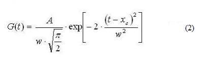
3.1. SG n - model. G U, i - peaks have the close parameters W and distances between peaks Δx i = (x c, i+1 – x c, i), and a considerable variability of their amplitudes, H i = A i / (w i · (√(π/2))) . U-data analysis shows, that G U, i - peaks are represented by two types of peaks, to wit by G U 1- type and G U A- type. G U 1- peaks have a small amplitude (H U 1 < 20) and so, they correspond to the single simple sunspot groups. G U A- peaks have amplitudes H U A > 20, which are changing in the broad range from ~ 20 to ~ 200, and so, they correspond to the active phase of the solar cycle with multiple sunspot groups of different complexity observed on the Sun. So, U-data is an alternating sequence of groups, consisting of G U 1- peaks or G U A- peaks. Groups of small G U 1 - peaks (they have the average length about 2.5 years) describe the periods of very low solar activity ("microscopic grand minimums", mGM) between the "active periods" of 11-year Schwabe cycles (S-cycles); in their turn, S-cycles (their active phase has the average length about 8.5 years) are represented by groups of G U, A- peaks with the changing amplitudes (see fig. 5 in [Kontor (2006)] ). It should be noted that the G U - peaks are one of the five types of quasi - regular temporary structures (QRTS), which can be distinguished in SSN time series. A typical G U - peak (QRTS 0 ) has the length of order of 1 year ( more specific TU = 2×w, see table 1 on the page "Data").
3.2. Analysis of K-data (K(t)), which are the very smoothed (filtered) M-data (they correspond to the frequency range [0 - f K:(1/4.17 (years), or 1/50 (months)] in the Fourier spectrum), allows to find out both the envelope of G U A- peak's maximums (H U A,i ) in each S-cycle and the "base smooth K - shape" of any S-cycle . Note here that S- cycle itself is the second from the mentioned above five types of QRTS of SSN time series. A typical S - cycle has the length of order of 10 years (QRTS 1 ). K-data are the result of M-data (pretty heavy) filtering , i.e. a smooth continuous quasi-periodic curve, which can be regarded as a sequence of S-cycles. However, it is known that this sequence of well observed S-cycles is sometimes interrupted by GM-periods during which solar activity is low, and the question of the existence of S-cycles is problematic. As SG 3-model has been developed to describe and forecast the so-called well-observed S-cycles, it is used when solar activity is developed enough, i.e. when the K-data exceeds a certain threshold (for U-data this limitation is less significant). Let us call periods, when the K-data <20, as GM - or mGM - periods (the latter are "gaps" between the well-observed S- cycles) and denote the corresponding to those periods K-data as K 0 -data. Then K-data can be represented as the sum of K 0 -data and K * -data. These last data > 20 and are pretty well described by SG 3- model; let us call this description # SGD:K, see (3) and fig.1:
(K i )*- data ~ # SGD:K (t 0, i ; t ) = Pi (t) + Bi (t) + Di (t) (3)
where t 0, i is the date of the S i -cycle (t) observed (or predicted) beginning and t 0, i < t < t 0, i +1 . It follows from (3) that any S-cycle is a superposition of three components of kind (2) - with the only exception in the face of # 4, which is described by four such components. In (3) i denotes the same as #, namely, a serial number of the considered S- cycle.
3.3. All G- peaks ( SG- model has three types of them (G U -, G K -, and G GL- peaks)) are different from each other only by the values of their three parameters: X c (the position on the time axis), w (width at half maximum, usually measured in months or years), and A = H · w · (√(π/2)), where H is the height of G - peak.
Consequently, the S-cycle's shape for each S-cycle is determined by nine parameters: X P, X B, X D (parameters of the time position, which are counted off t 0, i ); W P, W B, W D (the shape parameters, which are approximately equal and so designated by W), and at last H P, H B, H D ( "amplitudes" of P-, B-, and D - components of S-cycle). In accordance with SG 3 -model, eight from nine free parameters can be considered as approximately constant, and only one parameter (H P, i ) noticeably varies from one S-cycle to another. So, it is necessary to find out only the envelope of H P, i and to get after that the complete description (#SGD:K) of S-cycle K - shape (3) and the forecasts (#SGF: GL) for the next S-cycles (here they are #24, #25 and so on up to # 33) in the first approximation. So, H P, i - the height of Si- cycle's P component - plays a special role in SG 3- model.
3.4. SG 2 - model of GL-cycle. The long-term (~ 100 years) variation of Hp, i (t) is associated with the known Gleissberg cycle, which is considered in SG 2-model as a description of that variation. Then the Gleissberg cycle (GL- cycle) turns into superposition of two G GL- peaks (4):
#GL-cycle = G GL (t, X C , w 1, A 1 ) + G GL (t, X C+ Δx , w 2 , A 2 ) (4)
GL- cycle itself is the third from the mentioned above five types of quasi - regular temporary structures of SSN time series. A typical GL - cycle has the length of order 100 years (QRTS 2 ).
The whole Hp, i (t) - variation (GL-variation) itself can be described by the expression (5), see also fig.2:
GL-variation = ∑ G GL (t, (X C, i+1 = X C, i +Δx i ), w i , A i ) (5)
The mathematical expression for that envelope can be received from analysis of some SSN time series segment, which covers three Gleissberg cycles. It is the yearly averaged Y-data (1700 - present), and heavy smoothed (filtered) Y-data (E-data) corresponding to the frequency range [0 - f E : (1/17.86 (years)) in the Fourier spectrum] (see for details [Kontor, 2006, 2008 a]). Observations show that if the number of GL-cycles in GL-variation is integer, the odd Δx i ~ 41 years, whereas Δx i+1 ~ 63.3 years (even-numbered, giving the distance between the GL-cycles). We find that in norm the temporal distance between the adjacent G GL - peaks within GL-cycle is less than the "length" of G GL - peak (~ 55.2 years), whereas the distance between the adjacent GL-cycles approximately equal to the "length" of G GL - peak.
3.5. To receive an idea about variability of the amplitude of S-cycle's modulation, which is determined by GL-variation, it is necessary to consider SSN time series, which is longer than WSN time series, for example, LCN time series (9455 B.C. - 1995 A.D., see Solanki et al., 2005). LCN-data is close to E-data because they have the close Nyquist frequencies. Consideration of LCN-data from the point of SG-model's view shows, that three types (modes) of activity are realizing on the Sun: depressed (Grand minimum (GM i ) and mGM periods), when only the rare single sunspot groups (G U 1- peaks ) are observed for the some periods (it takes approximately 10 % of time); non - typical: the low S-cycles, in which the relatively stable B-component (3) dominates ( H P < H B > H D ) and the role of GL-modulation of the P-component amplitude (H P, i ) is inessential (it takes ~ 30 % of time inside Gleissberg cycles); and, at last, typical: the high (or regular) S-cycles, for which an amplitude is determined by GL-modulation (see for details [Kontor, 2006, 2008 a, 2008 b]). It takes approximately 60 % of time inside Gleissberg cycles).
3.6. SAE are the fourth from the mentioned above five types of quasi - regular temporary structures of SSN time series. Their lengths have a very large spread (from 200 to 2000 years), but as a reference the SAE length of order 1000 years (QRTS 3 ) could be considered (the shortest from the mentioned above five types of quasi - regular temporary structures is the structure, connected with the solar rotation (QRTS - 1 ); consequently it has the typical length about 27 days, or of order 0.1 year).
SG - model is just an instrument for investigation of SSN time series' and, specially, S-cycles' details, but we will see that it helps to understand qualitatively the temporal structure of SSN time series and variations of S-cycle shape in framework of contemporary Flux Transport Dynamo models. Mainly 3 of 5 structures are analyzed - QRTS 1 or S-cycle presented by K-data (see fig.1); QRTS 2 or GL-cycle as an envelope of H P, i (t) variation (see fig.2) and, at last, QRTS 0 or U-data (they could be the result of the transverse oscillations of the solar tachocline).
N. N. Kontor, e-mail: sgnnk@Live.com
first published: 11/27/2008
last published: 01/13/2020