This page displays my Forecasts for S-cycles # 24 and # 25. The previous pages discussed mainly the results of SSN - data' analysis using the SG -model. Now they allow the transition to the forecast of the 11-year S-cycle. We already have two types of auxiliary forecasts, namely, GL-forecast (i.e. H P, i (t) variation) for GL.4 - cycle (i.e. for S-cycles # 24 - 33, see fig.2 on page "Data") and WO - forecast for H m, i+1 (t), see fig.6 on page "Miscellanea". So, having analyzed the available data on S-cycles # (-4) - 23, I propose to use the following logic for forecasting of SSN - series using the SG-model: 1. Fixing the situation at the time of the forecast (t SGF), determining the possible types of forecast (GLL, GLS, GLS / WO) and the forecast horizon (t FН). For example, at the moment (t SGF = December 2019, 3252) GLL- forecast is possible for S-cycles # 26 - 33 to t FН = 2116 (see Fig. 2).
2. For S-cycle # 25, GLS - forecast is possible (more precisely, two forecasts (7.2) and (7.3)) up to t FН = June 2032, 3403 (see Fig. 4).
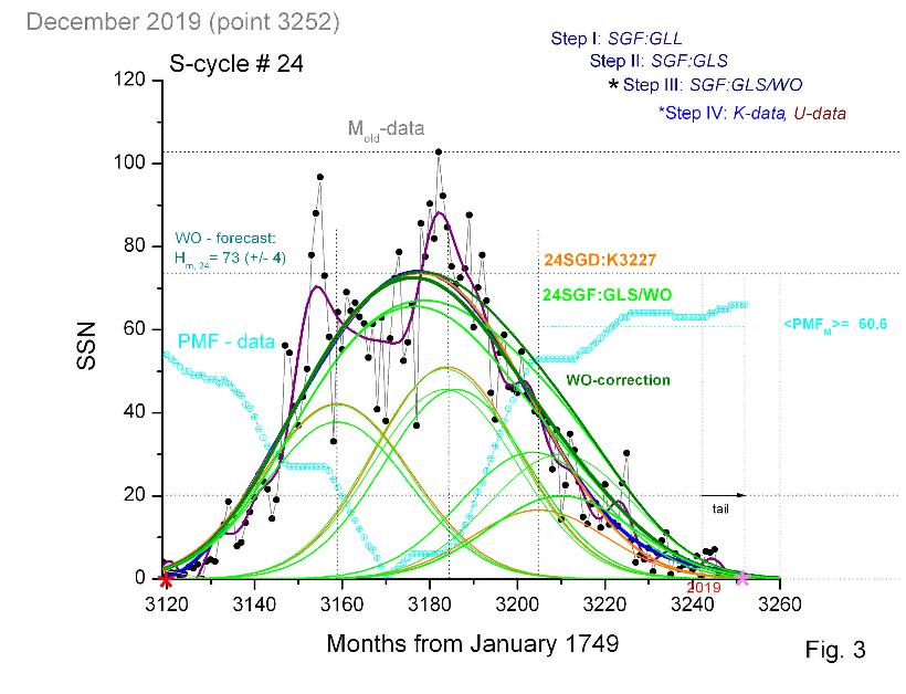
3. GLS / WO - forecast was made for S-cycle # 24 in May 2009, 3125 to t FН = August 2020, 3260. The forecast detail increases in the indicated order.
4. As M-data arrive, the forecast and observations are compared, which continues until the observed end of S-cycle (see Fig.3).
1. The first "SG - forecast" for S-cycle # 24.
The art of solar cycle prediction is unfortunately ambiguous. Our method of forecast is based mainly on SG-model (see pages "Model" and "Miscellanea"). SG-model is a tool for the study of solar activity, which is sensitive to factors such as: (1) a retrospective analysis of existing data; (2) the emergence of new data, both observational and theoretical; (3) at last, the process of matching the forecast with the incoming current data (M-data and others). This last factor implies prediction (#SGF:GL), which is made before the first M-data of a new S-cycle become available.
Elaboration of the SG-model was beginning in 2000, when the "Origin" software had appeared in my hands. The first and the only published (see Pesnell, 2008) prediction (24SGF.1) has been done in August 2006, which corresponds to the point 3092 in M-data time series (H m,24 = 70 (± 17.5) at t m,24 = 2012.96). The cycle's shape was being written as follows:
24SGF.1: {(3121+34.1)-28.7- (32×1.2533×28.7) = (3121+57.9)-38.6-(49×1.2533×38.6) = (3121+87.8)-32.6-(31×1.2533×32.6)}.
It fell on the decay period of the cycle #23, when, in principle, many parameters (which being requested for SG-model) of that cycle were known, excepting may be of the parameters of D-component (x D, 23 =3081, w D, 23 =39.1 months, H D, 23 = 20.4) and of cycle's length T 0,23 (151 months). Soon after the forecast 24SGF.1 has been done, the website on which the SG-model.2006 was described, has become unavailable and I made an unsuccessful attempt to publish SG-model.2006 in the "Solar Physics" (2008) journal. Then the new (this one) site has been developed (it has been launched in November 2008 - practically on the eve of S-cycle #24 start), on which in the real time three things are being made: the monitoring of S-cycle #24 current data; an analysis of those data on the base of SG-model.2006; and also the SG-model revision, which has been over (mostly, but not completely) as SG-model.C (current) or simply SG-model. The results obtained above in the description of the S-cycle's shape by the SG - model prove that those results are sufficient for constructing a GL-prediction of the next S-cycle. At that point it follows to note that SG - forecast (SGF) is being made in four steps: (1) long term regular (GLL), (2) short term regular (GLS), (3) comparison of the cycle's maximum using the PMF precursor (WO-forecast) and (4) M-data approximation (U).
2. Steps of predictions for cycles # 24, 25 and beyond.
Unlike some other forecasting methods, our forecast is aimed at a detailed description of the entire K-shape of the S-cycle. To emphasize "fundamentality" of the w-parameter in the SG - model, I note that you can first introduce the basic W-representation of S-cycle: w-w- H P, i = 2 w-w-2 w = 3 w-w-w, where w = 33 (months or dimensionless) and then can compare it with (6) on the page "DATA". However, experience shows that, due to the amplitude-time sensitivity of the SG 3-model, coarse initial representations of the shape of the S-cycle, which would seem to be used in the forecast, are not suitable, and, setting the initial form of the cycle, one should take into account as many of the available factors as possible. In particular, “average cycles” with an observed average duration of 132 months almost never occur; real S - cycles can be either short (T 0 ≈ 120 months) or long (T 0 ≈ 143 months), at Ϭ = 6 months. In short cycles, the closeness (see item 1 on page "MODEL") of the G-components increases (C <½), while in long cycles two effects are observed: it can decrease (C > 1/2) for the D-component and, in addition, a tail [τ], with the length about a year appears in some of the cycles . This (already the third) approximation-refinement is written as follows:
#SGF: GLL = t 0, i = 38.9 - 33 – H p, i (± σ) = 63.5 - 33 - H B, i = 90/100 - 33 – 20/30/40 =+[τ], (7)
GLL is the possibility of a long-term forecast, the main condition of which is the presence of the GL - forecast shown in Fig.2. For us, the S-cycle #23 was critical in this respect, until which the reliability of the GL 3.2 - forecast was doubtful. After H P, 23 was determined (approximately in 2002), it became possible to construct a GL-forecast for GL 3.2 and the entire GL 4 - cycle. This allowed, in principle, already then, to construct GLL- forecasts for S-cycles 24–33 (if we look seriously at our forecast from 1983 (Kontor et al., 1983), then from it follows that in the current SAE there will be only 5 GL- cycles ). However, the SG-model was just being developed, and in 2006, when 24SGF.1 was made, the time had come for the 24SGF:GLS forecast. So, for short S - cycles we have Tm = 90 + 33, i.e. 123 months ≈ 120 months, and for long - 100 + 33+ [τ] ≈ 143 months. Having SG 2 - the forecast for the GL.4 - cycle, shown in Fig. 2, you can get (# 26 - 33) SGF: GLL-s. In addition, one should not rely solely on the average H D,i = 30.5, because the shape of the decay phase (III) of S - cycle strongly depends on the height of D - component. This forecast, like everyone else, is subject to updating as observations become available.
2.1. Currently the start time of cycle 24 is of course known (December 2008, or point 3120), but for cycle 25 is not yet. Starting to build a 24SGF:GLS-forecast, we ask H P, 24 = 37.8 (from fig.2), H B, 24 = 45.6 (from (6.1)) and we face the problem of T 0, i.e. what should be the predicted duration of the S - cycle #24? When it comes to #SGF: GLS (for us they are S - cycles # 24 and 25), a fourth “approximation of analogues” is required when attempts are made to re-refine the predicted parameters based on a comparison of previously observed S-cycles having the same localization on previous GL-cycles.
2.2. To solve it, we use data about "analogues" and consider the corresponding sections of the GL- cycle. For cycle 24, they are D L -type cycles # 5 and 14, and for cycle 25 - E L -type cycles # - 4 and 6, as well as an anomalous U L- type cycle # 15. Cycles # 5 and 14 are similar: both long with tail; length, respectively, 151 months and 138 months; both follow the long D H -type cycles # 4 and 13. The cycle # 24 also follows the long # 23 and, according to the "logic of analogues", should have an average length of about 140 months. Then t 0, 25 = 3260, see fig.3 and (7.1).
24SGF: GLS =t 0, i = 38.9-33-37.8 (41.9) =63.5-33-45.6 (50.6) =90-33–20/30/40= {tail = 20} (7.1)
This cycle is assumed to be long (due to the tail) and low (HP <H B), as well as its counterparts # 5 and # 14 (therefore, x D = 90, not 100, and 20/30 were selected for H D). Then at its Тm = 123 months. should be expected [τ] ≈ 20 months. (this is a rather long tail). Since cycle # 24 has now almost ended, we can see that our forecast for the recession phase (IV) turned out to be the closest for the lowest D - component (under the condition H m × (73/66) - corrections for the WO forecast):
(3120)=3158.9-33-1563 (1735)=3183.5-33-1886 (2093) =3210-33-827/1241
2.3. The situation with S-cycle # 25 is less certain. For lack of other estimates, we start from 3260 and estimate X P = 3260 + 38.9 = 3298.9, and from Fig. 2 (3298.9 + 588) we determine H P = 37.5 (± 20) and the cycle type as a transitional S-cycle. In Figure 2, you can see only four such S-cycles (# - 4, # 6, # 15 and # 25). They are clearly different, although all are in the transition ("double minimum") region between adjacent GL-cycles. For the cycle # - 4, the ending S-cycle of the Maunder GM (1645 - 1715), M-data is still missing, but it still looks like cycle # 6 (low and long). Cycle # 25 could be the same if it were not for cycle # 15, which turned out to be abnormally high and short. The transition zone between adjacent GL-cycles seems to be unstable, since at this time the speed of the meridional circulation changes from small to large (and, accordingly, switching from long DS -cycles to short US - cycles). Therefore, for the cycle # 25, the following options are possible (see Fig. 4. GLS): (1) the low and long S-cycle similar to # 6 - 25 SGF: GLS (ll), (2) the low and short US - cycle similar to # 7 and # 16 - 25 SGF: 1, or (3) the high and short but abnormal S-cycle similar to # 15 - 25 SGF: GLS (h s).
2.4. So, for # 25 we'll have at least two options plus K-shapes of cycles # 6 and # 15 as they would look in the new M -data (see page"Miscellanea" and fig.4 GLS). For a low cycle, we select Н Р = 37.5 (± 20) from the GL - forecast (see Fig. 2). And for high Н Р it should be> 70/49 (the last number for the "old" spots).
25SGF: GLS/h s = t 0, i = 38.9-33- 70 = 63.5 – 33 - 69 = 90 -33-30/45/60 (7.2)
25SGF: GLS/ll = t 0, i = 38.9 -33 - 37.5 = 63.5 -33 - 60.5 = 100 -33 – 30/45/60 +tail=10 (7.3)
Then (assuming t 0, 25 = 3260) we get: (3260)3298.9-33-2895/1551=3323.5-33-2879/2502=3350/3360-33-1241
where the cycle's length will be about 120 or 143 months. Now the possibility of Grand minimum's start is almost excluded.
2.5. Knowledge of the PMF maximum, as it was established after pioneering works of H.W. Babcock (1961), A.I. Ohl (1966) and J.M. Wilcox, allows to predict the height of the next S-cycle prior to observations of its first sustainable high-latitude sunspots (i.e. before the cycle's start t 0, i+1). This type of prediction is considered now as the most reliable and theoretically confirmed (see Pesnell (2008), Petrovay (2010), Cameron and Schüssler (2015)). SG-model uses such an option for WO - forecast: <PMF M > is determined by averaging of current Avgf-data (Wilcox Solar Observatory data for the polar magnetic field strength, PMF) over the interval [x D, i - t 0, i+1 ]; then H m, i+1 = k * <PMF M > (see fig. 6 on page "Miscellanea"). It was possible during the decay phase of S-cycle #23 to evaluate <PMF M > = 55.5 (± 3) microtesla (cyan in fig.3). Then H** m,24 = 1.29 x 55.5 = 71.6; this is 24SGF: WO, which is close to both 24SGF.1 and 24SGF:GLS. #SGF: GLS/WO is an important comparison for #SGF: GLS using the latest observed data (<PMF M > and t 0, i+1). It allows you to not only specify a maximum of S-cycle (H m, i+1), but also its shape as a whole. PMF-data from Wilcox Solar Observatory (Avgf-data time series) were starting at May 1976. So, for # 22 we have H m,22 = 163.2 = 1.35 x <PMF M > (=121 (± 12)); correspondingly, for # 23 we have H m,23 = 121 = 1.2 x <PMF M > (= 101 (± 3)). Comparison of all currently available data allows to select the current compromise value of k = 1.29/1.84 (see fig.6).
2.6. Now it is possible to build U-data forecast SGF:U and compare it with M-data. It is supposed in # SGF:U that K- data represent the envelope for maximums of U-peaks, while the other parameters are taken from table 1 (page "DATA"). As data analysis shows there is a noticeable upward trend of H m, U i for U-peaks coinciding (or close) with the moments x P, i , x B, i , and may be, x D, i , i.e. moments of maximums of K-peaks shown in fig.3 by the dotted vertical lines. To emphasize this, the correspondent U-peaks will be increased by 30%; it follows that S-cycles actually should be three-humped (although for high S-cycles this tendency is less pronounced). The real U-data in fig.3 (wine line) show two of three expected peaks (compare with Karak et al., 2018).
3. analysis of deviations between forecasts and the current observations in the process of S-cycle evolution.
3.1. It concerns both K-data and U-data. As new M-data (grey points in fig.3) are coming they can be first partially and then completely compared with forecasts, and after that "the quality of forecasts" is analyzed. Technically it includes fitting of reliable data in some time interval by SG- model. Unlike the observed M-data, smoothed (filtered) data are unreliable both at the beginning of S-cycle (because during mGM period the Sun is still not active) and at the end of the available interval (because the future M-data are simply unknown). By definition the Sun is becoming active (only from that moment S-cycle is described by SG-model), when K-data begin to exceed 20 (for S-cycle # 24 that moment corresponds to the point 3138). To minimize the existing uncertainty, it is possible to consider as the future M-data 24SGF:GLS or 24SGF:U. As a result, it was obtained the following current description of the whole cycle #24 (blue K-data, compare with (7.1)):
24 SGD: K.3227 = {((3120 +38.9) - 33.7 - 42.2) = ((3120 + 63.9) - 32.8 - 51) = ((3120 + 84.9) - 30.8 - 16.6)}; Χ2= 0.029 (7.4)
This may result in shorter than expected cycle # 24.
3.2. For June 2016 we have: H m,24 K = 73 at September 2013; and H m,24 U 1 = 70.3 at Nov.2011 & H m,24 U 2 = 88 at Feb. 2014 (at the same time M-data also reach their maximum, 102.8). As for description of U-data, we get:
24 SGD: U.3204 = U 1, 24 (3120.45 - 3.3 - 4) + U 2, 24 (3131.6 - 4.93 - 8) + U 3, 24 (3141.3 - 9.3 - 19) +
U 4, 24 (3152.7 - 8.7 - 56.4) + U 5, 24 (3160.9 - 9.9 - 43) + U 6, 24 (3169.6 - 9.4 - 42) +
U 7, 24 (3181.3 - 10.35 - 78.3) + U 8, 24 (3191.9 - 10.35 - 55) + U 9, 24 (3202.5 - 7.9 - 36) + ... Χ2= 0.037
It can be seen from Fig. 3 that the phase of the decline of cycle # 24 somewhat ahead of the 24SGF:GLS, mainly because the D - component in 24 SGD: K.3227 (7.4) much lower than proposed in 24SGF:GLS.
3.3. Observations obtained in 2018 show that the activity of cycle # 24 continues to decrease gradually. In this case, the K-data goes slightly above the D-component's curve obtained in (7.4). This may mean one of two things: either the description of the K-data must be updated, or we are observing the beginning of the tail of the cycle (see description of Fig.1). Based on the structure of the SG - model and the phenomenon of cycle # 4, we can assume that the 11-year solar cycle consists of four activity waves - required, well known P -, B -, and D - components and t (D *). Into high cycles on the ascending branches of the GL - cycles (see Fig. 2), the P-wave sets the tone; B- and D-waves go in descending order, and the t-wave is practically absent. Therefore, these cycles are short (an exception - the cycle # 11). On the descending branches of GL- cycles, all four waves take place, but the peculiarity of such S-cycles is that they either have a relatively large delayed D-wave, which "absorbs" t-wave, or a t-wave degenerates into a shapeless tail (an only exception - of course, the cycle # 4). S-cycle # 24 looks not only low (as it should be), but apparently short (which is not supposed to).
Therefore, only the long tail can “save its reputation” (its analogs S-cycles # 5 and # 14 had tails 27 and 19 months long, respectively). Technically, the tail is observed as the noticeable excess of the U-data and K-data over (24)SGD:K (see (7.4) and the corresponding green curve in Fig.3) at the end of the cycle.
Nevertheless, as it said in "a Guidebook" on page "Miscellanea", the final comparison and conclusion can be made only after the current S-cycle's end, three consecutive attempts of prediction (GLL, GLS, GLS/WO) and the final description of the real K-shape of S - cycle.
3.4. The SG-model current expectations for the cycle 25 are shown in Fig. 4: GLS. Two 25SGF:GLS variants are shown, plus S-cycles # 6 (green) and # 15. All 25SGF:GLS-new will be compared with M new – data (see note A.5 on page "Miscellanea"). So, up to the current time, we have accomplished for S-cycle # 25 only Step (2). Nevertheless, already now (in October 2017 and later) you can make the current preliminary 25SGF: WO (for example, <PMF max> (for the period 3205 – 3234) = 58.9; so H** m,25 should be 58.9×1.84 = 108 (see fig. 4: GLS)).
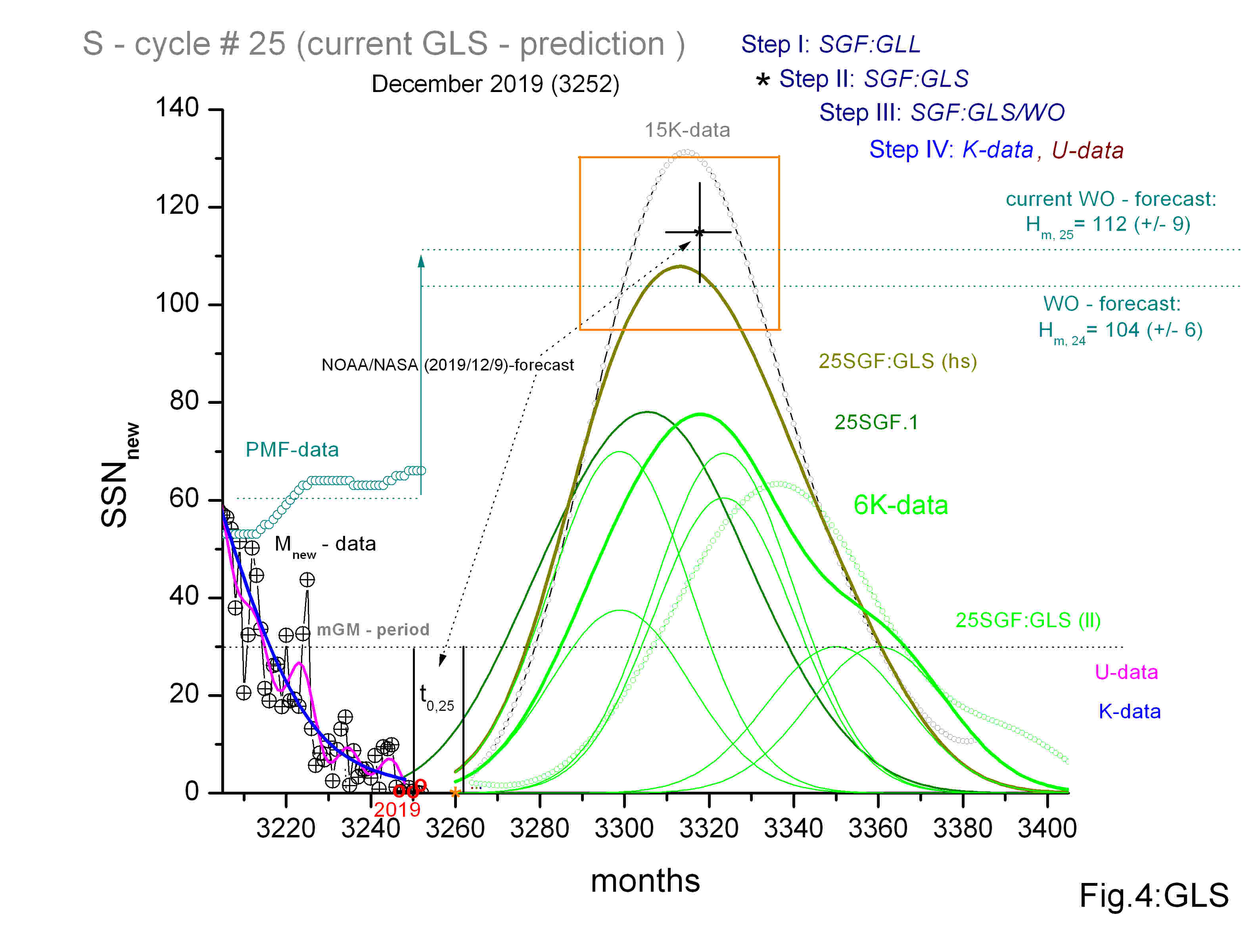
3.5. Figure 4: GLS shows that today the situation with the forecast of the 25th cycle is still quite contradictory. This is due to the assumed position of the cycle 25 within the Gleissberg cycle (see Fig.2). The fact is that it is in the region of the extremum (specifically, at the minimum) of the GL - cycle. Observations show that in the region of the extrema of the GL - cycle, the probability of development of anomalous S - cycles is markedly increased (see S - cycles # 12, 15, 19, and probably 25). Therefore, in Fig. 4: GLS, there were all four possible types of forecasts: (1) the absence of a S - cycle due to the onset of a Grand minimum (see Ref.2018/1 and current extrapolated behavior of K-data and U-data); (2) emergence of a critically low S - cycle (see 25 SGF: GLS2 (7.3) and #6 K - data); (3) emergence of an intermediate S - cycle (see 25 SGF: GLS1 (7.2)) and (4) emergence of a high S - cycle (see #15 K-data). By the way, the current WO - forecast still remains somewhere in the middle between options (3) and (4), and the orange square shows the consensus reached by experts in April 2019.
3.6. However, not everyone, unlike me, is staying before the problem of S - cycle # 25 forecast in deep thought, like Knight at the Crossroads in artwork by Victor Vasnetsov (1882). For example, Prantika Bhowmik & Dibyendu Nandy (2018) indicate that "based on our simulations, the corresponding prediction for the yearly mean sunspot number at the maximum of solar cycle 25 is 118 with a predicted range of 109–139. The maximum of solar cycle 25 will occur around 2024(±1). The range of ±1 year also includes the uncertainty in the exact timing of cycle 24 minimum which may vary by 6 months". This means that their forecast corresponds to our high forecast and short S - cycle, which is similar to cycle #15. Then they conclude that "our ensemble prediction indicates the possibility of a somewhat stronger cycle than hitherto expected, which is likely to buck the significant multi-cycle weakening trend in solar activity. Our results certainly rule out a substantially weaker cycle 25 compared to cycle 24 and therefore, do not support mounting expectations of an imminent slide to a Maunder-like grand minimum in solar activity".
3.7. I am currently analyzing the course of mGM - period, shown in figures 4 and 7 (see item 6 on page "Miscellanea"). It is clearly seen that over the past three months (November, December, 2019 and January 2020) an increasing activity of S-cycle 25 has been observed (red circles in Figs. 4).
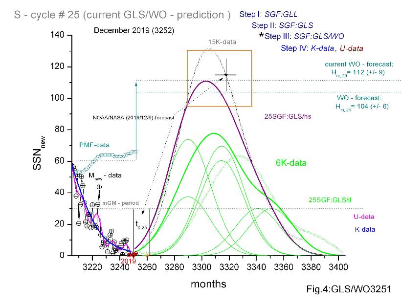
Given the current situation, when the activity of the new S-cycle # 25 clearly exceeds the activity of the old S-cycle # 24, I assume that t 0, 25 = 3251 (November 2019) and do the first 25SGF: GLS / WO / 3251. For the low and long cycle 25SGF:GLS/ll we get H m = 78, t m = 3309 (September 2024) and Tm = 143 months, while for the high and short cycle 25SGF:GLS/h s - correspondingly H m =111, t m = 3303 (March 2024) and T m = 123 months. Since the current WO-forecast gives H m = 112, I assume that S-cycle # 25 will be abnormally high (in the scope of my SG - model) and it will be a precursor of a high GL.4 - cycle just like S - cycle # 15 was a precursor of ours GL.3 - cycle (see fig. 2).