Appendix and References

1. Site Content

1. Page "MODEL" includes 3 parts

2. Page "Data" includes 8 parts, Fig. 1, 2 and table 1.

3. Page "Miscellanea" includes 6 parts and Fig. 6, 7, 9

4. Page "Forecast" includes 3 parts, Fig. 3, 4

5. Page "Conclusion" includes 3 parts, Fig. 5 and tables 2 and 3.

6. Page "References"

2. A Guidebook through SG-model SSN time series superposition of Gaussians (SG -) model

SAE (a Solar Activity Episode), see Solanki et al., 2005; Usoskin, 2008; and (4,5) on the page "Model".

GM (a Grand Minimum of solar activity, for example, "Maunder GM" (1645 - 1715))

GL-cycle (a special kind of the Gleissberg cycle), see fig.2

GL-peak (any one of two components of GL-cycle)

S-cycle ( 11-year solar cycle)

M-data (monthly averaged sunspot numbers (SSN))

U-data (a slightly smoothed M-data), see (1) in the page "Model"

K-data (a very smoothed M-data)

The normal (Gaussian) presentation of S-cycle's components, see (2) on page "Model"

P-, B-, and D- components (see (3) on page "Model" and table 1 in the page "Data") of K-data (K-peaks)

U-peaks of U-data

See parameters of K- and U-peaks in tables 1 and 2 on pages "Data" and "Conclusion"

TMF - bunch is a hypothetical concentration of a strong toroidal magnetic field (TMF) in the tachocline region.

PMF is the large scale weak poloidal magnetic field on the Sun.

SCB is the Solar Conveyor Belt of large-scale meridional circulation in the Sun (Hathaway, 2010).

BLH - mechanism of PMF formation in the FTD - models (see part 5) is based on corresponding papers of Babcock, H. W., Leighton, R. B. and Hathaway, D.H.

SG-model forecasts (#SGFs) - # means a S-cycle's serial number.

"Climatology": S-cycles can be of 7 types - UH/L - cycles (among them EH - cycles) , DH/L - cycles (among them SH - cycles) and E L - cycles. Each type has the own specific shape. For example, << S (D L) >> is

37 - 32 - Hp,i = 65 - 35 - H B,i = 89 - 32 - 30 (these are cycles # 5, 14 and possibly 24); or << S (U L) >>, which is

35 - 32 - Hp,i = 56 - 33 - H B,i = 84 - 34 - 25 (these are cycles # 7, 15, 16 and possibly 25); or << S (E L) >>, which is

48 - 33 - Hp,i = 74 - 33 - H B,i = 100 - 33 - 20 (these are cycles # - 4, 6 and possibly 25).

Another version of the same classification contains only 3 types of S-cycles: US-cycles (include UH/L - cycles and EH - cycles), DS-cycles (include DH/L - cycles and SH - cycles), TS-cycles (include E L - cycles and AS-cycles).

The height of P-component follows GL-cycle, shown in fig.2.

#SGF: GL(L/S) - this type of the primary forecast actually is a more or less long extrapolation made before the beginning of the next S-cycle. It based on averaged previously received parameters. For example, 24SGF:GLS was made in 2006, two years before the S-cycle #24 real beginning, and 25SGF:GLS was made at the end of 2015. As for "classification", #SGF:GL includes features of climatological, spectral (and statistical) forecasts.

Right after fixation of the new S-cycle start, the secondary "precursor type" #WO-forecast is made. It allows to compare the predicted heights of the next S-cycle. Furthermore, on its base the opportunity for #SGF:U appears.

Those four kinds of forecasts deplete the predictive potential of SG-model relatively S-cycle. At the same time we should not forget about the possibility of GL-cycle's extrapolation (GL#:F). For example, at the current time attention is focused on the GL_4 - peak's shape (see figs. 2), i.e. on GL_4:F.

During S-cycle evolution an exciting time of comparing predictions with observational data coming exhausts the nerves. Simultaneously recognition of discrepancies and trials of their explanation definitely contribute to the improvement of the model. Nevertheless, the final comparison can be made only after the current S-cycle's end. It consists in comparison of the forecasts with the final S-cycle descriptions by #SGD:K (description of K-data) and #SGD:U (description of U-data), and its analysis.

3. U - data as approximation of M - data

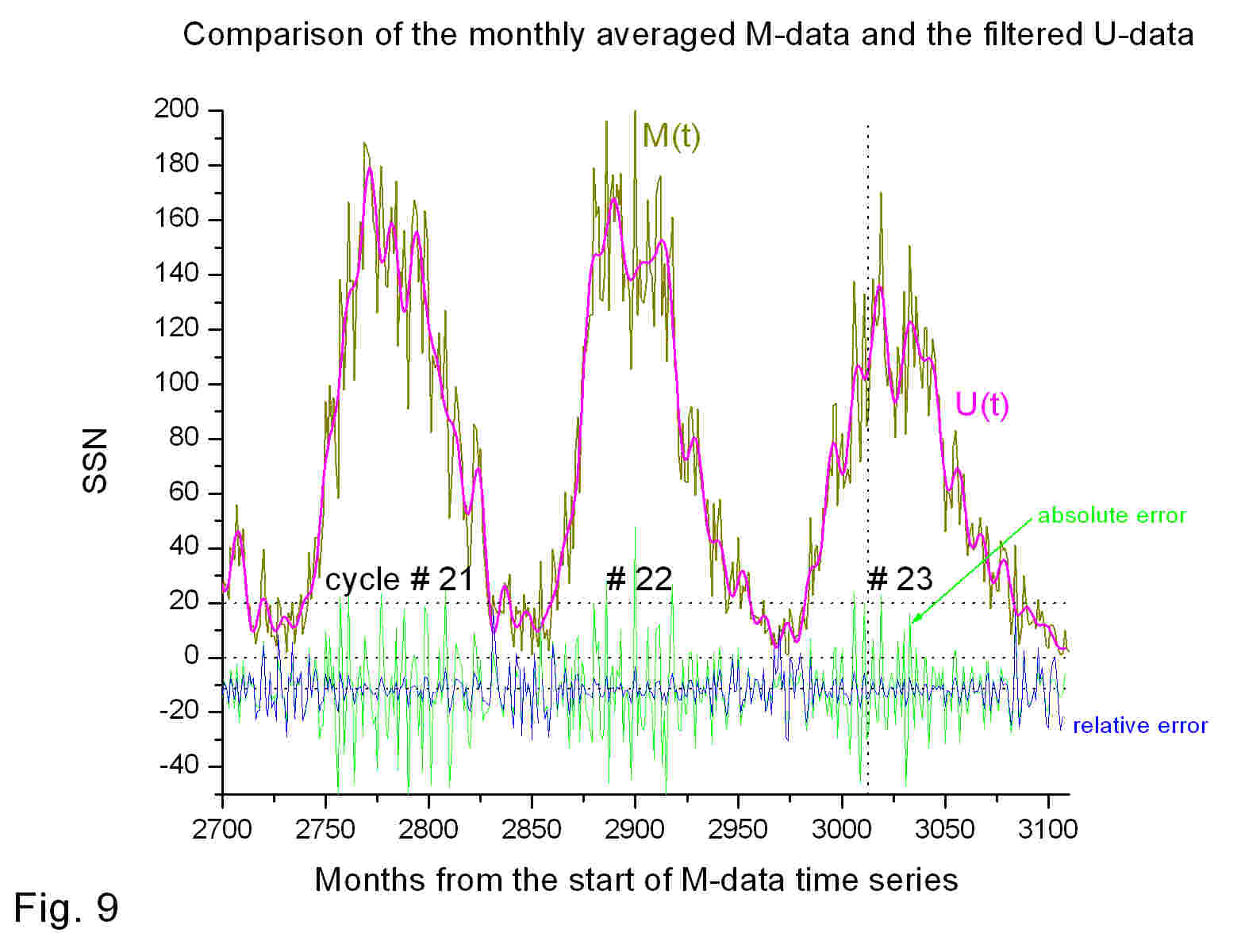
A1. σ = 11.83 (1) is just an estimation of random scattering of M(t) around U(t). The real comparison of M-data and U-data behavior is shown in fig.9.

A2. SG-model described here is carefully considered in Kontor (2006, 2008a and 2008b), and its critic can be found in Kontor (2008c). Particularly, anticorrelation of X D, i and H P, i is shown in fig.13 [Kontor, 2008a].

4. WO - method basics

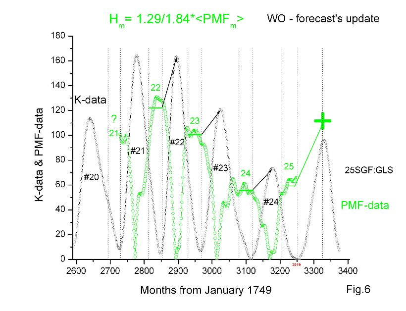
A 5. 2015 - a year of great change in SSN data. Announcement from WDC - SILSO: "Since July 1st 2015, the original Sunspot number data are replaced by a new entirely revised data series... Data Credits: The Sunspot Number data can be freely downloaded. However, we request that proper credit to the WDC-SILSO is explicitly included in any publication using our data (paper article or book, on-line Web content, etc.), e.g.: "Source: WDC-SILSO, Royal Observatory of Belgium, Brussels". Thus, now at our disposal there are two types of SSN - data - the old (R. Wolf's, for example, M OLD - data) and new (for example, M NEW - data) ones. Those data have a good linear correlation - (M NEW - data/M OLD - data) = 1.427, what helps to transit from one type to another and vice versa. Using M O - data, I have got GL - variation shown in fig. 2. It shows "the position" and H_P_{, i of}S_i- cycle. It allows (on the table 1 & 2' basis) to get 24 SGF: GL forecast or K*- data. After that, using the WO - forecast' idea, H**_m_{, 24}= k (=1.29) · <PMF> (=55.5) can be received. As M_o– data become available (after t _0,24= 3120 (Dec. 2008)), an opportunity of K-data and U-data receiving becomes also available . So, 24 SGD: Kt and 24 SGD: U t could be received. However, in 2015 SSN were predetermined so that new M_N– data = 1.427 · M_O- data. But since by that time S - cycle # 24 has surely overcome the maximum, it makes sense to finish it on the basis of M_O- data. As for S - cycle # 25, it should be already described "in the language" of M_N– data. For that "the old" 25 SGF: GL should be multiplied by 1.427, and then (when the time comes) H**_m_{, 25}= k _N (1.84 (=1.29 · 1.427)) · <PMF> could be received. For that you first need to calculate "the new" GL _N – variation, beginning from S - cycle #23 (multiplying the corresponding interval of "the old" GL - variation to 1.427). Then everything goes according to the old algorithm, but with the new M-data (see fig.6).

5. Flux Transport Solar Dynamo current understanding.

Solar dynamo problem bothers physicists for almost a century . After fundamental ideas of Larmor (1919), Cowling (1933) and Parker (1955) the long period of search of the realistic dynamo models and ratio between advection and diffusion in the processes of generation and transfer of the magnetic fields in the convective zone has come (Petrovay, 2010). Helioseismology (Kosovichev, 2011) has made and is making major adjustments to the theoretical understanding of the structure of the CZ: its lower boundary ( tachocline ), DOUBLE-CELL MERIDIONAL CIRCULATION pattern (Zhao et al., 2013), properties of the upper subphotospheric granulation layer. Given the increasingly complex picture of the processes in the CZ and on its borders, one should be more attentive to the observed variations in solar activity, including variations of the solar cycle (S- cycle) shape, in an attempt to associate these long ( for centuries ) observed variations with new ideas about the structure and processes in the CZ. As the SG- model shows, the parameters of S-cycle's shape are quite stable, what allows to develop a fairly accurate prediction of SSN time series. However, the reasons for the stability as well as significant deviations from the forecast can be understood (and, consequently, predicted) only on the basis of an adequate physical model of the solar dynamo . The immediate prospects for the development of such a model are described in Karak et al. (2014): “Over the past few decades, kinematic mean-field and FTD models have developed in parallel to MHD simulations, unfortunately with relatively little cross-fertilization. On the one hand, because of their relatively modest computational requirements mean-field dynamo models, such as FTD, are likely to remain the workhorse of investigations regarding solar cycle prediction, and the modulation of solar activity on long timescales, including Grand Minima. They also offer a computational framework within which to investigate efficiently the joint action of turbulence and flux emergence, albeit in simplified form. This can provide useful guidance for the design of MHD numerical simulation of the solar cycle, in which systematic exploration of parameter space is impractical. Numerical simulations, on the other hand, can provide quantitative constraints on key transport mechanisms and source terms currently implemented in a largely ad hoc manner in most kinematic models. They can also provide crucial information on the dynamics of large-scale flows important for dynamo action, which is inaccessible to kinematic models by their very design. Cross-fertilization is mutually beneficial, and this review has attempted to identify areas where this could be most productive in the context of FTD models. A true unification of FTD models and convective dynamo simulations can only come about through an improved understanding of flux emergence. Elucidating how convective dynamos produce emergent toroidal flux structures through the combined effects of rotational shear, magnetic buoyancy, and turbulent transport is a prerequisite to clarifying the role of flux emergence in the origin of magnetic cycles. Does flux emergence play an essential role in the operation of the solar dynamo, as in FTD models that rely on the Babcock-Leighton mechanism, or is it merely a superficial by-product of deeper-seated dynamics, as suggested by the presence of magnetic cycles in current MHD convection simulations lacking emerging sunspots and active region? From the perspective of the four dynamo ingredients (identified in Sect. 5.1), this is perhaps the most pressing. We can summarize the central issue with a more general restatement of the BL paradigm: how can the process of flux emergence promote the generation of a mean poloidal field? Though MHD simulations may not achieve a comprehensive depiction of the solar dynamo in the next decade, they can and will provide new insights into this central question, together with increasingly sophisticated FTD models and continuing observational scrutiny of solar magnetism and large-scale flows. Progress on this front has recently been reported by Yeates and Muñoz-Jaramillo (2013) who presented a novel 3D kinematic FTD model with an algorithm for flux emergence inspired by MHD simulations and calibrated with solar observations. The ideal test bed for investigating the relative roles of the BL mechanism and convective field generation (as modeled by the turbulent α-effect) may be Grand Minima . In particular, convective field generation may account for the residual cyclic activity during the Maunder Minimum (Beer et al. 1998) and may provide a mechanism for pulling the Sun out of a Grand Minimum. Other areas where the synergy between MHD simulations, FTD models and solar observations may potentially yield trans-formative insights in the coming decade include magnetic flux transport , the more general manifestations of solar cycle variability (including but not limited to grand minima and grand maxima; and the linkages between large and small-scale dynamo action”. Incidentally, I hope that the results, obtained with using of the SG- model, can be used in the developing of such an adequate physical model of the solar dynamo .

6. S-cycle # 25 start time.

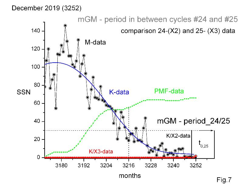
According to the FTD - model (see part 5), cycle # 25 began to be developed from March 2013 (point 3171), when, after a period of polarity reversal, the “new” PMF, which was being formed by the BLH - mechanism, appeared in the sun (see Fig. 7, a green curve). Over the next three and a half years (44 months), cycle #24 (black circles) passed from the phase of maximum (III) to the phase of decline (IV), PMF was growing, but no other signs of cycle #25 were observed in the sun. Then short lived "ephemeral sunspots", belonging to cycle #25, have been reported on Dec. 20, 2016; April 8, 2018; Nov. 17, 2018; May 28, 2019 and July 1, 2019. And only on July 8, 2019 (point 3247) was registered AR # 2744, which record-keepers will likely mark as the first official sunspot of cycle #25 (see red curve). But by this time both cycles were at the phase I - mGM (24/25).

It begins at December 2016 (3216) and until June 2019 (3246) only "old" sunspots of the cycle # 24 are observed. The first ("new") sunspot of the cycle # 25 appeared, as already said, 2019 - 07- 07 (3247, AR 2744/25). From this moment, in principle, any new spot could become a benchmark for the beginning of cycle #25.

It should be noted here that the period under consideration belongs to the rare type of "double minimum", when mGM falls on the period of the minimum between adjacent GL-cycles (see fig.2).There are only four such double minimums in the current SAE. The first took place between S - cycles # - 4 and # - 3, when the Maunder minimum was replaced by the first GL1- cycle; then there were no sunspots for two years in a row; I attribute the center of that mGM to January 1712. The second took place between S - cycles #5 and #6, when the GL1- cycle was being replaced by the GL 2 - cycle; then there were no sunspots for more than a year in a row (639 days); I attribute the center of that mGM to August 1810 (close to the start time of S-cycle #6 on December 1810). The third double minimum took place between S - cycles # 14 and # 15, when the GL 2- cycle was being replaced by the GL 3 - cycle; then there were no sunspots for 92 days in 1913 year in a row (total this year had 311 spotless days) ; I attribute the center of that mGM to May 1913 (close to the start time of S-cycle #15 on August 1913). The current fourth double minimum has its mGM (24/25) center at t 0,25, which is still not known to us. Up to now so far (2019-12-31) it looks pretty modest: 2019 has 281 spotless days and only 40 spotless days in a raw. In other words, this minimum so far looks the least deep (more precisely, the least wide) of all the four "double minimums" that have been observed so far.

Our goal is to determine t 0,25 so early as it possible. But this is not July, when the first AR 2744/25 appeared, because during the next three months only "old" AR/24 (# 2746 - 2749) were observed. Then, maybe this is November (3251), when two new AR/25 (#2750 and 2752) and only one old AR 2751/24 were observed? To answer this question, you need to look at what will be observed in December and later. Conclusion for the first half of December 2019: according to data for July - November, old ARs prevail in quantity, frequency of occurrence and M-data. But in November, new ARs prevail. So, to, 25 will arrive no earlier than November 2019 (see also reference: SOLAR CYCLE 25 FORECAST UPDATE: December 09, 2019.

The NOAA/NASA co-chaired, international panel to forecast Solar Cycle 25 released their latest forecast for Solar Cycle 25. The forecast consensus: a peak in July 2025 (+/- 8 months), with a smoothed sunspot number (SSN) of 115 (+/-10).

Additionally, the panel concurred that solar minimum between Cycles 24 and 25 will occur in April 2020 (+/- 6 months)).

At the end of December 2019, two ARs belonging to cycle #25 were visible on the Sun. Since early January 2020, the southern AR 2755/25 has dominated on the Sun.The last gap between the new ARs was 5 days, while the old ARs did not appear for more than 63 days. Therefore, according to today t 0,25 = 3251 (November 2019, nine months ahead of my forecast). However, the further course of SSN is quite capable of changing this preliminary result. Let's wait and see, but so far (on January 6, 2020, when the Carrington rotation (CR) # 2225 ended) there are only signs of an increase in the activity of S-cycle #25 (see figs 4 & 7).