1. Time series which have been used.
On this and the following pages, the background of SG-model, data used and the procedures of their analysis, the results, forecasts mainly for S-cycles # 24 and 25, and their relevance to the modern scenario of the solar cycle are explained.
Here is the list of data which are the sources for SG - model:
1.1. M - data (January 1749 - May 2015) include S - cycles # 1 - # 24 (M old - data) and M new - data (after May 2015) for S - cycle # 25 and so on (WDC - SILSO, Royal Observatory of Belgium, Brussels).
1.2. U - data are (slightly) filtered M - data (include the periods > 10 months).
1.3. K - data are (heavy) filtered M - data (include the periods > 50 months). By the way, K-data are more smoothed than conventional 13-month boxcar averages (M 13-data).
1.4. Yearly averaged Y - data ( 1700 - 2015) include S - cycles # (- 4) - 23, i.e. 28 S - cycles.
1.5. Averaged LCN - data (9455 B.C. - 1995 A.D.) include about 30 SAEs (see Solanki et al., 2005).
1.6. E - data are the filtered Y - data (include the periods > 18 years).
1.7. Daily D - data (1818-1-1 - 2015-5) are used for Fourier analysis of the high frequency features of SSN time series.
2. SG 3 - model basics.
The results of analysis of each of these time series have contributed to the solution of our problem, namely, to the quantitative description of a structure of the time series of solar activity, which is represented by SSN time series. Our SG-model of the SSN time series is developed on the base of two main assumptions that seem to me reasonable and promising: (I) smoothed (more specific - filtered) SSN-data can be described by some superposition of Gaussian functions G(t) (2) and, in particular, (II) S-cycle (represented by K-data) can be described by the superposition of three G(t) with true to type width 2 w (for each), which is equal to the period of the first harmonic (5.5 years) of the main peak (11 years) in the Fourier spectrum of SSN time series. It follows that w in (2) should be equal in average 33 months. And everything else - as it will.
So, it is known that the main structural element of the SSN time series is the 11-year solar cycle (S - cycle). For the analysis of its form (shape) we will use K - data. Usually when it comes to a particular S - cycle, we refer to its number and settings such as the start date (t 0, i), date of maximum (t m ) and the value of this maximum (H m), and the date of the end of the cycle (this date is, at the same time, the start date (t 0, i+1) for the next cycle). SG-model allows to describe the shape of the cycle significantly more detail. Immediately it should be said that the numerical value of any parameter of S- cycle is known with some (sometimes long) delay (for example, the start of cycle #24, which took place in December 2008, became known in May 2009). Therefore, any substantive discussion on the current cycle implies some kind of forecast. In order to lay the basis of the forecast of the solar cycle, SG-model has been introduced (see page "Model") and on its basis all of the above series, including each of the 23 cycles presented in M -, U -, and K- data, were analyzed. As an example, fig.1 displays a description of the longest S-cycle # 4.
3. S - cycle # 4' case.
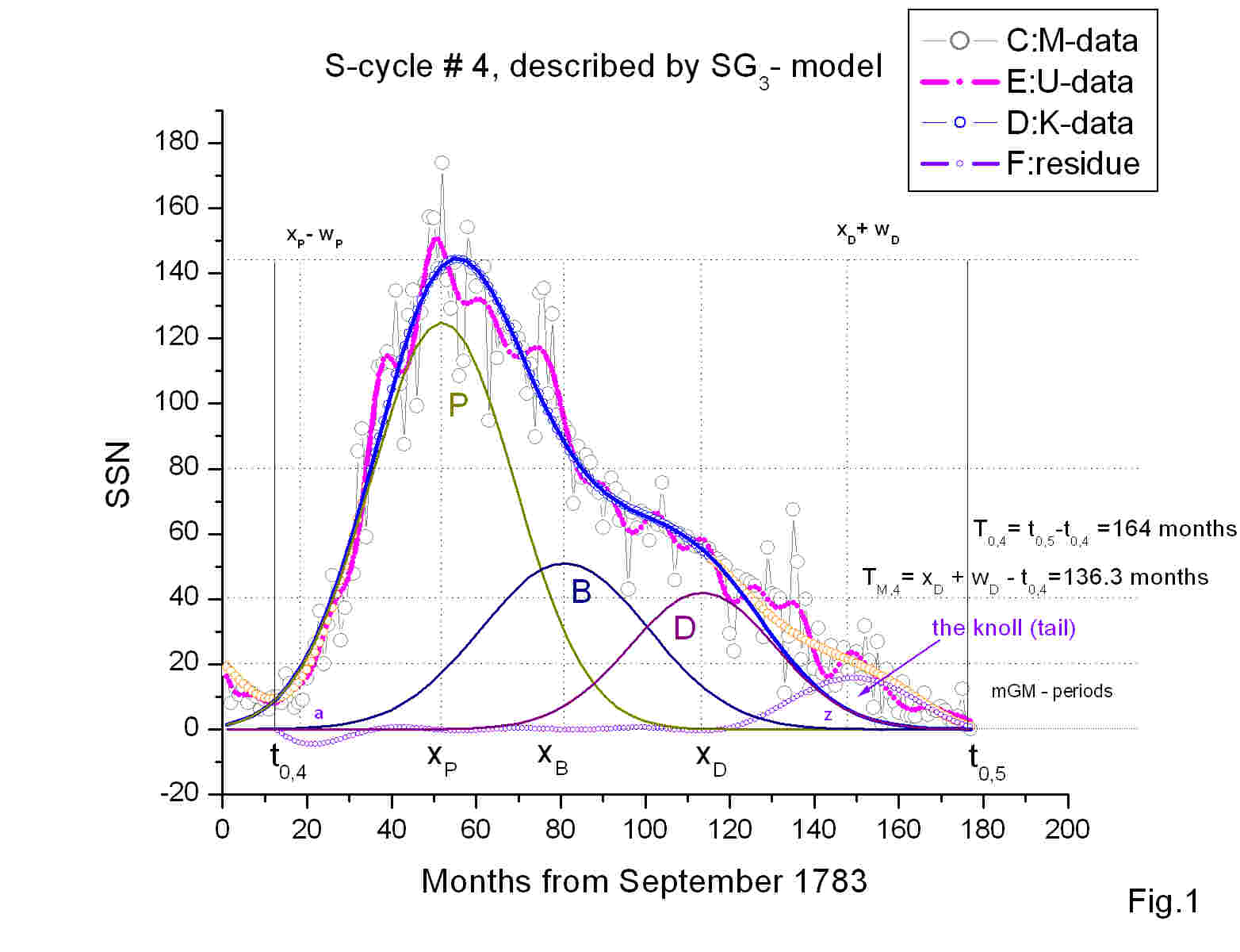
3.2. Important moments and parts of S - cycle: it consists of five distinctive parts and includes 10 important reference moments. It starts at t 0, i ("the moment" 1) inside the mGM - period of low activity (the first part), which separates the neighboring S - cycles. It is possible the simple and convenient description of the mGM - period's length as the time interval, when K - data < 20. In that case the average length of mGM - period (and consequently K 0, i - data) = 35.4 ± 17.9 (months), i.e. in average it is about three years. But the observed range of its changes is [20 - 89 (months)]. After the end of mGM - period ("the moment" 2) an active part of S - cycle begins. It has duration about 8.15 years, which corresponds to a "sub-peak" of the main 11- year peak in Fourier spectrum of SSN time series. An active part of S - cycle consists, in turn, of three periods - an activity growth (the second part) , when P - component is emerging (it may include the moment x P (3), whereas the moment (4) means the start of the cycle maximum (the third part), when B - component is evolving (it includes the moments t PR (5), t m (6), x B (7) and (8), which means the start of the cycle's decay (the fourth part) - the time of D - component (it includes x D (9) and (10), which means the start of new mGM). During transition to the next mGM - period sometimes small humps at the end of cycle (the single knolls) can observe (the fifth part). The cycles with a knoll have usually a long duration. Thus, the expression (3) may differ markedly from K 0, i - data during the mGM-periods, while they are practically the same (K* i - data) in the active phase of the S-cycle (5). Therefore, to distinguish between K-data and their description using (3), let us denote (3) as #SGD: K. So, any S-cycle in SG-model can be presented by M-data (observed), U-data (filtered), K-data (filtered), #SGD: K and #SGD: U (both fitted); wherein U-data and #SGD: U are practically identical. All the above applies to any S-cycle, including S-cycle # 4.
3.3. S -cycle # 4 started in September 1784 ( t 0, 4 = 12 in fig.1) inside the current mGM - period. All data are shown after that moment up to May 1798 ( t 0, 5 = 176). "The moment 2" takes place at point 21. After that the active part of S - cycle # 4 begins. It is seen that an activity growth is determined mainly by P - component (x P = 51 what is close to t m = 56 ; at that time the moment of t PR was unknown). The moments of x B = 74 and x D = 108.4 correspond to the cycle's decay period. It is interesting to note that the moments x P , x B and x D approximately correspond to "the splashes" of activity, seen in M- and U- data. It explains the double peak shape observed in some S-cycles (#1, 9, 10, 11, 15, 19, 22, 23). It is S-cycle # 4 in which the most massive hump at the end of cycle (the single knoll) can be seen. It is seen very good in graph of residue = K-data - 4SGD: K, see (3) , fig.1 and table 2. The attentive reader will notice that for a good description of the K - data, a massive masking (mm) of the initial and final parts of the S - cycle is required (see yellow points in fig.1). To decrease mm up to the level K - data < 20, you can allow the output of one or even several parameters outside ± σ. However, for # 4, since it is anomalous already because it is the longest, it was possible to describe it as a superposition of not three but four normal components: P, B, D, and D* (compare with (3)). It looks like #4 is {39 - 33.6 - 116 = 62 - 37.7 - 52.6 = 96.4 - 36 - 48.6 = 134.6 - 32.9 - 14.2}
P-component B-component D-component D*- component
The example of fitting the cycle # 4 well shows the difficulties that arise in the description of K-data by SG - model. As a result of numerous (I'm not afraid of this word) fits gradually came the idea of a satisfactory algorithm of adjustment (fitting), taking into account the necessary restrictions. However, to prove that the algorithm is the only one, I still can not.
4. Fitting Algorithm (FA). Normally the fit goes in several stages:
(1) The initial cycle is set more or less arbitrarily:
= position parameters (Xp, Xb, Xd) are selected by means of averages, if there are no additional instructions for their selection;
= height parameters (Hp, Hb, Hd), as it turned out, are related by two correlations:
Нв = 35 + 0.28 * Нр (сс = 0.93) and Нd = 24.6 + 0.1337 * Нр (сс = 0.55); the second relation is not used further, it is giving just for information.
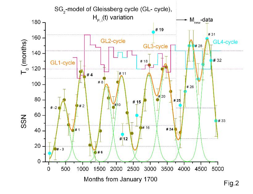
= parameter Hp has a special status: its variation from cycle to cycle is (in SG-model) regular and describes GL-cycle (see Fig. 2). It is assumed that this is the essence of the GL-cycle;
= shape parameters (Wp, Wb, Wd) are chosen equal to 33 months and first fixed.
(2) the K-data fit is first reduced to the "landing" of the source cycle on the data using the position and height parameters within approximately one error;
= thus the volume of obvious masking of the beginning and the end of K-data is clarified, and the reached chi-square is fixed.
(3) After that, the shape parameters are activated for the fit, and the constraints on the parameter values are amplified;
= Now the fit is in all 9 parameters;
= As the values of the parameters are extended to allowable boundaries (± 2 Ϭ), additional masking of the beginning and end of the K-data is carried out until χ2 < 0.1;
= If all efforts are futile (χ2 > 0.1, or the deviations of the parameter/parameters are more than two sigma, or a massive masking of the beginning / end of the cycle is required), the cycle is recognized as anomalous and the appearance of its anomaly is established. At this end a description of the cycle is considered complete.
Figure 1 shows the results of fitting the longest cycle # 4 to a superposition of three Gaussians P (t), B (t), D (t), which is used for all other cycles. Typical deviations of K-data from the model at the beginning and end of the cycle are shown. However, for # 4, the best description is a superposition of four Gaussian P (t), B (t), D (t), D * (t). Table 1 shows the mean values obtained for each parameter (and some additional results). Figure 2 shows the GL- cycle (variation of Hp, i) and its variants following from the model. Table 2 shows the parameter values for each S-cycle, beginning with # 1 (see page "Conclusion").
5. SA is some observed effects of the functioning of a complex MHD - system formed in the convective zone of the Sun. The behavior of the sunspots and their number (SSN) is characterized by a mixture of regularity, randomness and chaos, in which both determinism, such as the laws of nature, and uncertainty, and the suddenness of the blind case are seen. All this can be seen in the behavior of the SSN - series, in which the sequence of 11-year S-cycles is suddenly replaced by the GM - period, and then somehow is restored. But the S-cycles themselves differ markedly in form, which, it seems, somehow reflects the current mode of operation of the solar dynamo. What are these differences? In short, these are differences in the height, duration, and form (shape) of successive S-cycles. The first two are observed directly, and the shape of the cycle is determined by its model. In our SG 3 - model, the elements of the S-cycle structure are:
(a) a quasi-regular variation in the height of the first (P) G-component (see fig.2);
(b) the lag of the active phase of the cycle relative to its observed start;
(c) the presence of an irregular "tail" in the cycle, which distorts the regular shape of the third G-component and affects the duration of the S-cycle (see the cycles # 5, 6, 11, 12, and 14);
(d) the degree of description (estimated in %) of the cycle by the model. It turns out that there are no identical S-cycles, but there are similar ones.
For the purposes of forecasting, it is desirable to have a classification of S-cycles, i.e. a description of the observed types of S-cycles. There are two of them: short (120 (+/- 6) months) U-type cycles and long (143 (+/- 9) months) D-type cycles.
In this case, we can distinguish sub-types of these two types:
ascending {U (L / H) - # 7, (15), 16 & 2, (11), 17; and extremely high E (H) - # 3, 8, 18, (19), 21, 22};
descending {D (H / L) - # 4, 9, 13, 23 & 5, (12), 14, high saddle S (H) - # 1, 10, 20; critically low E (L) - # (-4), 6}.
They differ in height, in length and in shape, in particular, in the absence or presence of a long (~ 16 months) tail.
6. SG 3 - model's constraints. Due to many free parameters (9, remember J. von Neumann ?), the fitting procedure is ambiguous: any S-cycle can be described equally well ( i.e. practically with the same chi-square (Χ 2)) by several different sets of parameters. To remove that ambiguity, certain constraints were imposed on the fitting procedure itself. Here they are.
1. All w i should be close to 33 months (in average w = 33.1 (±2.7), w P = 33.2 (±2.7) , w B = 32.6 (±2.1) , w D = 34.1 (±2.5)). 2. Model's S-cycle length TM = x D + w D should be close to the observed length of S-cycle T 0 (Δ2 = T 0 - TM = - 0.11 (±3.4) m, i.e. really close, but excluding cycles # 5, 6, 11, 12, and 14. For them Δ2 = 21 (±4.8) m). 3. For pretty high, positively asymmetric S-cycles, P-component is the main component, i.e. the highest one (S-cycles # 2, 3, 4, 8, 9, 10, 11, 13, 17, 18, 19, 20, 21, 22, 23). 4. For pretty low, symmetric or negatively asymmetric S-cycles, B-component is the main component, i.e. the highest one (S- cycles # 1, 5, 6 (symmetric), 7, 12 (symmetric), 14, 15 and 16 (both symmetric)). 5. P- and B-components generate the cycle amplitude, whereas D-component is responsible for the cycle's length. 6. Fitting procedure concerns only the active part of S - cycle; thus the start and end portions of K-data (that is K 0 -data substantially belonging to mGM periods) are excluded from fitting (by masking, see a- and z- "components" in fig.1).
The first step deals with fitting of P- and B- components to the growing and maximum phases of the S-cycle (under condition: P-component should be as high as possible for the high, positively asymmetric S-cycles, and vice versa: B-component should be as high as possible for the low, symmetric and negatively asymmetric S-cycles); the second step deals with fitting of B- and D-components to the decaying phase of S-cycle; and the third one matches both previous so as to obtain the good Χ2 . 7. Fit is considered good (indistinguishable to the eye), if Χ2 < 0.1 (average Χ2 = 0.061 (± 0.026)).
All 23 S-cycles, being fitted, have allowed to get table 1. Some results of this work are presented in tables 1 and 2, in comments to those tables and shown in fig.1 and fig.2.
7. Table 1: Estimations of some average SG - model parameters
PARAMETERS | X C | σ | ΔX | σ | W | σ | H | σ | |
U-data
G U - peaks | G U A- peak | - | - | 10.8 m | 14 % | 8.48 m | 13% | > 20 | - |
G U 1- peak | - | - | 12.0 m | 10 % | 6.57 m | 18% | < 20 | - | |
K-data
G K - peaks | G P - peak | 38.9 m | 4.9 m | - | - | 33.2 m | 2.4 m | 78.6 | 39 |
G B - peak | 63.5 m | 6.5 m | - | - | 32.7 m | 3.0 m | 57.0 | 11.8 | |
G D - peak | 92.8 m | 9.7 m | - | - | 32.9 m | 2.8 m | 30.5 | 9.2 | |
- | - | - | - | - | - | - | - | ||
E-data
| G GL - peak
| - | - | 41.8 y | - | 27.6 y | 18% | 109 | 11% |
63 y | 13 % | ||||||||
LCN- data
| G GL - peak | - | - | 46 y | 24 % | 31.65 y | 13% | - | - |
7.1. The average values of main parameters of SG - model are shown in table 1. They were received by the entire array of data for all 23 S-cycles. "m" means months; "y" means years; "-" shows that the corresponding parameter can not be characterized only by the average value, or just is not relevant to the case.
7.2. Taking the average parameters (from table 1), one can write symbolically the average S - cycle (< Si >) as follows:
< Si >= {((t 0, i +38.9) - 33 - Hp,i (± σ)) = ((t 0, i+63.5) - 33 - H B,i) = ((t 0, i +92.8) - 33 - H D,i = 30.5)}, (6)
where H B,i = 35/50 + 0.28 * Hp,i (6.1)
8. Gleissberg-cycle in SG - model.
8.1. It is also seen from table 1 that parameters w P, w B, w D, x P , x B and x D are the most stable; other two parameters H B, and H D are "intermediate" stable, and only one parameter H P looks like unstable. If to show the variation of H P,i (t) on the graph (see fig.2), one can see that H P,i (t) changes cyclically and that rhythm (cyclicity) looks like the famous Gleissberg cycle. Because the leading role in SG-model is given to P-component (see constraint # 3), we assume that it is the dynamics of the P-component is a major factor (but not the cause) of the Gleissberg - cycle occurrence. Let us call this "special" representation of Gleissberg-cycle as GL-cycle.
8.2. Fig.2 shows 8 GL-peaks describing the variation of the H P, i (t). SG 2 -model describes GL-cycle by two humped curves. The first S-cycle has the number - 4, the last - number 33. "The anomalous cycles" and "cycles under forecast" (# 25 - 33) are shown as cyan circles. GL. 3-cycle is not over yet, but it is not excluded that it may happen during the S-cycle #24; GL-peaks #7 and 8 (GL. 4-cycle) are our forecast on the basis of the average GL-cycle. Errors for all S-cycles are taken equal to ± 14; they include both physical (including variability of unknown parameters of the poorly understood mechanism of the solar cycle) and instrumental (including ambiguity of the fitting procedure) errors. Two horizontal lines (solid and dot) are seen in the low part of Fig. 2. The solid line corresponds to the border between high and low S - cycles. Zone below 20 (dotted line) is a critical one, where the flip to the Grand minimum (GM) is most probable. The corresponding E L - type of S-cycles occupy "the lower saddles" of GL-cycles (see # - 4, 6, and probably 25). A regular GL-cycle has well-defined lower and upper saddles (see # 1, 10 and 20 cycles belonging to S H - type), ascending cycles (see UH/L - type # -3, -2, -1, 2 and 3; 7, 8, 11, 12; 15, 16, 17, 18, 19, 21 and 22) and descending cycles (see DH/L - type # 0, 4, 5; 9, 13, 14; 23 and 24). As for the real GL-cycles (shown in orange in fig.2), they usually have a "deformed" shape, when maximums are unequal and some S-cycles (see # 12, 15 and 19) fall out of the "normal" course of GL-cycle.
8.3. An analysis of SSN time series and S-cycles in particular, which is describing here, has the ultimate goal of developing the solar cycle prediction techniques. So, we should have an idea about the behavior of the solar cycle's parameters. There are two kinds of such parameters: "amplitude" (H P, i , H m, i , H B, i , and H D, i) and "temporal" (t 0, i, x P,i , t m, i, x B,i , x D,i , TM,i and T 0,i ). From these 11 parameters the last one is the most mysterious. The estimate of the cycle's length (T 0, i) and conditioned by it the next cycle's start (t 0, i+1) becomes difficult, if not hopeless case. The fact is that evolution of S-cycle takes place in three relatively independent stages. Each of them can be associated with a magnetic harness at the bottom of the convective zone, "emitting sunspots". The first in time harness begins to produce sunspots at a relatively high solar latitudes (~ 30 degrees). A SSN - course in this period (an activity growth ) is described in SG-model by P-component. The second harness starts especially intensively to produce sunspots in the period of the cycle's maximum at latitudes of about 15 degrees. A SSN-course in this period ( the cycle's maximum) is described in the SG- model by superposition of P - and B - components. Then begins the downturn of the cycle (the cycle's decay) and its behavior is determined by at least two factors: production of sunspots by the third harness at the latitudes ~ 8 degrees (this factor is described in SG-model by D-component) and the effectiveness of the process of sunspot magnetic field reconnection in different hemispheres (North and South) in the equatorial zone of the Sun (this process is observed in the form of more or less rapid decline in SSN during transition from the active phase of the cycle to mGM - period). Thus it appears that the behavior of the decay phase is weakly associated with the phases of growth and high activity in the S-cycle. For example, very high cycles (# 3, 4, 8, 18, 19, 21 and 22) are usually short; however, cycle # 4 was not just a long, but the longest one. Distribution of S-cycle's duration has a sophisticated look, which I tried to be reduced to two types of S-cycles: the short ones, <TS> = 119.5 ± 6 months (in the range of 108 - 126) and the long ones, <TL> = 142.5 ± 6.5 months (in the range 135 - 151). So, the average duration <T 0 > = 132.4 ± 14.7 months falls within the range from 127 to 134, in which S-cycles are not observed at all. Thus, you can make more or less successful attempt to estimate the length of the current S-cycle with a precision of ± (6 -7) months, taking into account all available reasons, however, it should be understood that in the framework of the SG - model we will be able to know it for sure only six months after t 0, i+1 real coming. The more advanced analysis shows that the length of S- cycle takes one of three values: T 0,S ~ 120 months (10 years); T 0,L ~ 138 months (11.5 years); and T 0,L+ ~ 150 months (12.5 years). To advance somehow in the question of S-cycle's length, let us assume, that GL-cycle reflects not only the amplitude variations of S-cycles, but also their temporal characteristics, i.e. the S-cycle's shape as a whole. Let us formulate this assumption as follows: "S-cycles arranged on GL-cycle similarly, have approximately the similar shapes" .
That assumption allows to distinguish three base types of S-cycles: ascending (U - cycles), descending (D - cycles) and E L - cycles, see above, comment 4. As data show, those types correspond to the "compact" short S-cycles (U H # 2, 3, 8, 17, 18, 19, 21, 22; and U L - # 7, 15, 16) with T 0,S ~ 120 months; and to the "delayed" (shifted) S-cycles "without tail" (S H # 1, 10, 20 and D H # 13 with T 0,L ~ 138 months; and D H - # 9, 23 with T 0,L+ ~ 150 months) and S-cycles "with tail" (# 11, 12, 14 with T 0,L ~ 138 months; and # 5, 6 with T 0,L+ ~ 150 months). Fig.2 also shows the variation of cycle length (T 0) in relation to the GL - cycle's course. It's enough to enter to the forecast of the next S-cycle. The description of the GL-cycle by normal peaks is convenient, but does not reflect the fact that S-cycles of U-type are short, and S-cycles of D-type are long. Therefore, the ascending part of the GL-peak should be shorter than the descending one. The description of the GL-cycle with log-normal peaks (asymmetric peaks with σ ~ 0.1) indicates that the average duration of the GL-peak's growth phase is 264.8 months, while the recession phase - 328.8 months. (difference of 64 months); if there are three S-cycles in the growth and decay phase, then the difference will be ~ 69 months. I assume that the long-term forecast for the averages is meaningless and one must go from cycle to cycle; more precisely, it is necessary to continuously adjust the super-long-term forecast. Nevertheless, in Fig. 2 such a regular over-long-term forecast for the GL4 -cycle is shown (for cycles # 25 - 33 (predicted T 0,S =120 months and T 0,L=143 months are also shown (cyan))).