1. Techniques, Results, Predictions...
1.1. Introduction. The most general notion used here is solar activity. It includes a generation of large-scale toroidal (TMF) and poloidal (PMF) magnetic fields (solar dynamo), their inter conversions, the slow (magnetic diffusion) and fast (reconnection or solar flares) their dissipation and a whole set of the other observable solar phenomena (the 11-year solar cycle (S-cycle) of sunspot number (SSN); Grand minimum (GM) of solar activity; the Gleissberg cycle (GL-cycle) and so on). The fact is that a mathematical basis for understanding the solar activity is the system of Navier - Stokes and magneto-hydrodynamics equations , which consists of nearly two dozen equations. It is clear that such a complex system of equations can not be solved in the forehead, and it is required the significant simplifications of it (leading to a loss of some essential physics). Such simplifications, for example in the theory of the solar cycle, indeed have been made, see Ossendrijver, 2003; Nandy, 2009; Parker, 2009; Olemskoy, 2014, Kumar et al., 2019. However, for the elaboration of a theory, the prompts or constraints that it receives from observations are necessary. These are observed effects that can not be ignored. Such effects are Hale's magnetic polarity law; Spörer’s law; S-cycle's length; some helioseismic results; Joy's law; GM existence and a number of others. Science develops when curious observers and experimenters throw up facts that dodgy theorists explain with the help of their theories and even get consequences, which after are searched for by these very observers and experimenters. Studies of solar activity are not an exception to the rule.
Trying to bring my contribution to the study of solar activity, I must first describe the logic of SG-modeling of the SSN time series. The SG-model of the SSN time series was conceived with the aim of accurately describing the regular form of the 11-year solar cycle (S - cycle). After considering the Fourier spectra of the known SSN time series, three types of SSN - data were taken for analysis: monthly average M-data, their weakly smoothing filter (U-data with period cutoff <10 months) and a strongly smoothing filter (K-data with period cutoff <50 months). A comparison of the form M - & U - data is shown in Fig. 9. The regular form of the S - cycle will be called K * - data (3). In the SG - model, they are described by the SGD - function: K (t) with χ2 <0.1 (see Table 2), which is almost indistinguishable by eye. SGD: K (t) represents a superposition of three Gaussians G (t) (2), and the main of the three parameters of each G-component is its “half-width” W ≈ 33 months, the value of which we assume is equal to half the period T ≈ 5.5 years, observed in the Fourier spectrum of the SSN time series. In this case, the expected "length" of the S - cycle is T 0 = 33 × 4 = 132 months (under the condition of "closeness" of the Gaussians C = ½), which is almost equal to the average duration of the S-cycle. However, such “average cycles” actually are not observed, rather, S - cycles can be either short (T 0 ≈ 120 months) or long (T 0 ≈ 143 months), at Ϭ = 6 months. In short cycles, the "closeness" of the G-components increases (C <1/2), while in long cycles two effects are observed: it can decrease (C> 1/2) for the D-component and, in addition, a "tail" with length about a year appears in some of the cycles.
The most variable of all nine parameters of the S-cycle shape (see Table 1) is the height of the first G-component H P, i. Figure 2 shows its changes from one S - cycle to another S - cycle. If we describe them as a sequence of GL - peaks of the same form (2), we obtain a special form of the two - humped Gleissberg - cycle (GL - cycle). It shows ascending and descending S - cycles, as well as the deep "double minimums" that separate GL-cycles (1711/1712, 1810, 1913 and the current - 2019/2020).
1.2. Data. In this situation, I am in the crowd of observers who dream to put out of countenance those arrogant theorists. But I do not know if they will notice me (I certainly mean the results presented). I started in 1998 from that to describe the shape of any solar cycle (represented by (yearly averaged) Y-data) by a one-humped asymmetric smooth curve (it was a log-normal curve). The result was unsatisfactory. Then I made the transition from smoothed to filtered data (using Fourier series) and received along with the regularly observed M-data, U - data and K-data. U-data are slightly smoothed in comparison with M-data and may be used as some approximation (1) of abruptly changing M-data. K-data are more smoothed than the generally accepted smoothed M13-data and it allows to get the good (indistinguishable to the eye) description of the active phase for any S-cycle. Another preliminary result was the realization that the first harmonic (5.5 years) of the main (11-year) peak in the Fourier spectrum of SSN time series can be related to w (width parameter) of G-peaks (2), superposition of which describes the shape of the S- cycle represented by K- data. From consideration of 23 observable shapes of S- cycles it followed that the smallest number of G-peaks, included in this superposition, is 3. It meant that the number of free parameters should be equal to 9. It was the price to pay to obtain the low Χ2, i.e. the good (indistinguishable to the eye) description of the S-cycle shape. It allowed to get the table 2 of all parameters for all 23 available cycles. SG-model assumes that the solar cycle is a superposition of, at least, three one-humped symmetric curves (G-peaks (2)). The page "Data" displays the average values of main parameters of SG - model (table 1). This provides a description of the regular shape of a particular S-cycle, its regular forecast, and even the regular SSN time series. In using the term "regular", I mean such a state of solar activity, which is not distorted by stochastic/chaotic fluctuations of SG-model's parameters (which, of course, take place in reality).
Table 2 of S-cycle's parameters (#SGD)
A B C D E F G H I J K L cycle #
75 48.8 36 40.6 73.9 33 48.1 103.5 33 39.5 135 0.052 1
210 34.3 32 72.6 54.6 33 52.4 79.8 29.4 41.1 108 0.059 2
318 36.7 29.3 116.5 57.5 29.7 63.9 87.3 26.5 28.6 111 0.087 3
429 37.7 32 109.8 60.4 35.7 65 95.6/132.2 33.7/35.8 49/19.1 164 0.088 D* 4
593 40 31.8 25 70.3 36 37.7 92.8 31.2 18 151 0.037 * 5
744 48.5 33 14.4 73.5 33 36.4 100.6 33 14.2 149 0.075 * 6
893 47.6 33.9 39.9 75.7 31.5 45.2 95.7 27 39 126 0.015 7
1019 36.1 29.9 107.8 56.9 26.9 62.3 83 32.6 41 116 0.08 8
1135 44 37.5 82.5 69.5 38.8 59 109.7 33.4 37.6 149 0.05 9
1284 43 31.7 70.4 66.3 32.7 53.6 103.8 35 39.6 135 0.07 10
1419 39 32 103 62 30.6 59.3 92 33 26 141 0.06 * 11
1560 32.8 33.9 35.5 58.1 31.3 50.3 84.1 34.4 25.8 135 0.035 * 12
1695 35 34.8 63.4 60.4 35.7 46.7 103 35.9 19 143 0.052 13
1838 33.6 31.5 36.8 59.3 34.9 41.1 85.6 33.6 30.4 138 0.007 * 14
1976 41.3 34.4 60 63.2 33.9 52 92.9 32.5 14 120 0.033 15
2096 35.2 33 44.1 57.6 33 51.5 85.2 33 25 122 0.017 16
2217 43 32.1 79.7 65 31.7 66.3 97 31.7 37.7 125 0.056 17
2342 43 32.5 125.1 65 29.6 64.6 90 30.5 46.3 122 0.038 18
2464 41 33.5 167.6 64.2 31.8 84.3 95.5 32.5 33.1 126 0.084 19
2590 40 35.4 80.3 67 37 66.7 103 38.6 38.6 140 0.04 20
2730 39 32.4 120 59 28.5 72.5 83 34 61.6 123 0.029 21
2853 34 31.2 122.4 54 28.1 68.2 75 34.4 52.9 116 0.026 22
2969 45.5 39.6 90.9 72.9 35.5 64.3 111.5 38 20 151 0.046 23
col (A) - t 0, i (months from the beginning of M-data series (January 1749)); col (B) - x P,i , col (C) - w P, i, col (D) - H P,i ; col (E) - x B,i , col (F) - w B, i, col (G) - H B,i ; col (H) - x D,i , col (I) - w D, i, col (J) - H D,i ; col (K) - T 0,i ; col (L) - Χ2. All parameters (except H P,i ; H B,i ; H D,i ; and Χ2 : they are dimensionless) measured in months.
1.4. SG - model scope. Not trying to convince a reader of any special benefits of the proposed approach and not hoping to protect myself from the inevitable criticism (which is not always constructive and often is directed by the human factor), I represent here some results.
First of all, it is H P,i (t) variation (see col (D) in table 2 and fig.2), which can be described (in accordance with the adopted approach) by the sequence of GL-peaks (2), the temporal distance between which changes periodically (from long one to short one and vice versa). Consideration of fig.2 allows to see in this sequence of a "Bactrian camel" of the Gleissberg cycle (GL-cycle).
It is seen from fig.2 that S-cycles in their positions on GL- cycle (which is actually represented in fig.2 as one of the possible images of the Gleissberg cycle) can be ascending of the type U (including maximum), or descending of the type D, or saddle ones (wherein the saddle cycles occupy either the upper (#1, 10, 20) or the lower tier (# - 4, 6, 25?).
It is obvious but very important that each of those types of S-cycles is characterized both its peculiar shape, and duration ((T 0,i ), see the page "Data"). From the point of view of possible deformations of S-cycle's shape, they can be "compact" (it concerns mostly the ascending cycles), "shifted" and / or "tailed" (this applies to both descending and saddle cycles, but not to all).
It is this last result allows transition of S-cycle's forecasts from the method of "averages" ("av-method", when only H P,i (t) is predicted while other parameters are taken average, see table 1) to the method of "analogs" ("an-method", when only parameters of related similar cycles are compared). Experience has shown that it significantly improves distinctness of some forecasts, while for others the "av-method" is more preferable .
The joint analysis of K-data and U-data would complement the S-cycle forecast #SGF:GL.L/S, represented only by K-data (see fig. 3, 4), by the S-cycle forecast #SGF:U, represented by U-data (see fig. 3). The U-peaks, approximately coinciding with the moments x P,i , x B,i , and x D,i , can be sometimes increased by 1.3 times as compared with other U- peaks, the height of which is determined by the value of K-data (K- data represent the envelope for maximums of U-peaks). Using (1), #SGF:U may be compared with the current M-data (a different approach is proposed in Karak et al., 2018).
Another result is the possibility of working out a mutual option of "GL- and WO- forecast". SG-model shows that PMF reaches the maximum <PMF max > during the period between x D,i and t 0,i+1 . Averaging PMF-data (Wilcox Solar Observatory Polar Field Observations, Avgf - data) for that period, we receive <PMF max,i >, which can be connected with H m,i+1 .
1.5. A diverse phenomenon of solar activity is apparently a side effect of a plasma dynamical system, which is formed in the solar convection zone (and on its borders) and probably is in a state of weak chaos. SSN time series is just one of the observable manifestations of solar activity. And although, to my knowledge, the chaotic origin of SSN time series is not yet proven, its behavior, at first glance, looks very irregular. However, on closer examination, one can find in SSN time series some regular temporal structures, which are described in the SG-model by three types of G-peaks (2),
namely, G GL-peaks with w ~ 28 years (they describe the regular behavior of Gleissberg cycles);
GK-peaks with w ~ 33 months (they describe the behavior of regular 11-year solar cycles),
and GU-peaks with w ~ 30 weeks (they describe a regular component of the SSN fluctuations with the period of 1.3 years).
Since the MHD system of the solar convection zone that generates the solar cycle (and much more) is not only complex, but also difficult to observe, the SG - model relies not so much on theory as on the analysis of available and continuously incoming data (in fact it is M-data and < PMF> - data). So, SG-model is not a physical, but a phenomenological model, in which the elementary methods of mathematical statistics are used. There is no visible physics in it, but basic physical concepts about the origin of solar cycle lay down in its base. The issue here is not that I, being a physicist, want to do without physics, but the fact that the physics of the main elements of SG-model is still insufficiently known. Indeed, there is no appropriate physical model of the Sun's Great Conveyor Belt (SGCB or SCB), which apparently determines the behavior of the Gleissberg cycles; there is no discussion about three-component structure of the 11-year S-cycle; there is no physical model of the 1.3-year oscillations, which are clearly presented in the U - data.
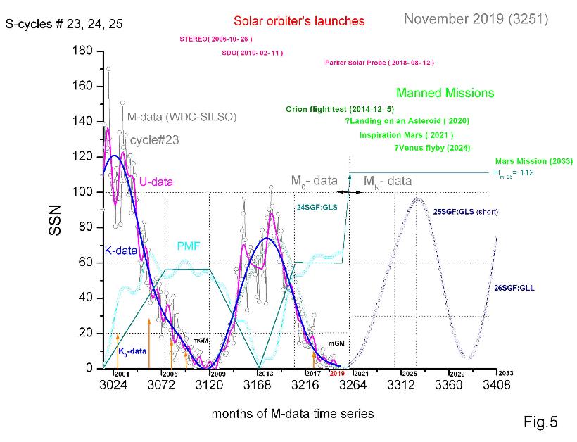
The fact is that (according to some sources) the horizon of predictability for the solar cycle is only a few years, and so any attempt to build a long-term forecast of S-cycle looks unprofessional. From the other side, to have such a forecast is very interesting (and in some cases, very important). Here the President Eisenhower's aphorism, applied to such a complex system as the human society, comes to mind: "plans are useless, planning is priceless". Replacing one notion by another close one, it would be to said with respect to the solar activity: "forecasts are useless, forecasting is priceless". Indeed, "wittingly doomed" attempts to forecast S-cycles have led to detection of a number of connected features of solar activity, which ultimately lead to better understanding of the S-cycle and properties of the SSN time series. Working with the SG-model for more than 10 years, I was convinced in this from my own experience. The hope is that the SSN time series is only weakly chaotic, and therefore it is possible to consider SSN time series as a regular process with a slightly fluctuating parameters of the elements of solar activity (in the SG-model it is G-peaks) and relatively rare anomalous deviations from regularity (indeed, of 23 S-cycles, only three (cycles # 12, 15 and 19) are really anomalous). Fig.5 illustrates the view of the recent solar activity and its forecast from the standpoint of the SG-model on the background of solar research projects and the projects of manned missions in the hither heliosphere. By the way, if the planned flight to Mars takes place, it will take place during the period of high activity of S-cycle #26 (if, of course, instead of S-cycle #25, a new GM-period does not begin, what we will soon find out).
1.6. Results. So, what do we learn applying SG- model to SSN time series?
I must say that in the study of solar activity, there are two aspects - practical and theoretical. They, of course, closely related, but there are differences. The practical aspect aimed to use the beneficial properties of the SA and to protect from its negative effects, and its main mean is the expanding of monitoring of solar activity, space weather and so on (Kontor and Somov, 1998). At the same time the theoretical aspect aimed on the solution of solar mysteries, one of which is the nature of the solar cycle. This puzzle exists more than a century and it was not resolved even during such a creative 20-th century; therefore it moved into the 21-st century, along with associated general physical problem of turbulence and mathematical problem of solving of the Navier - Stokes equations. Generally speaking, it is known that science adheres (until a certain time) some paradigms and science is subject to fashion. For the solar cycle a paradigm is "MHD - dynamo" (see Ossendrijver (2003) and Charbonneau (2010)) and a current fashion is "Flux Transport Dynamo" (FTD) - models (see Choudhuri (2012), Olemskoy (2014)), Kumar et al. (2019) "in which the toroidal field (TMF) is produced by differential rotation in the tachocline, the poloidal field (PMF) is produced by the Babcock - Leighton mechanism at the solar surface and the meridional circulation (SCB) plays a crucial role". And this role is to arrange the solar activity (particularly for us - the structure of SSN time series) in a large scale (across the whole convective zone) and in the long term (about 10 S-cycles, or one Gleissberg cycle). Working with the SG-model, we are able to indirectly monitor changes of TMF in the tachocline (variations of sunspot numbers (SSN)), changes of PMF on the surface of the convective zone (using WSO observations) and, as we shall see below, changes of the mode of meridional circulation (or the Great Sun's Conveyor Belt (SCB or simply CB)).
Let's start with small scale and will move towards ever larger scale. We miss the shortest from the mentioned above five types of quasi - regular temporary structures, connected with the solar rotation, and immediately turn to the U- data, which can be described by G U, i -peaks ((2), see also table 1). These peaks have a width at the base TU =2·w = ~ 17 months, but partly overlap and their closeness C = [ΔX/(2·w)] = ~ 0.64. Origin of G U, i -peaks could be spatial (if you imagine that TMF in the tachocline splits into bundles and meridional circulation (CB) occurs across them (see Kontor and Khotilovskaya (1988) and Kontor (1991)), temporal (connected with transverse vibrations of the tachocline (see Howe et al. (2000)), or mixed.
The next quasi-regular temporary structure is 11-year S-cycle, which consists of three G K -peaks (see tables 1 and 2). Every G K -peak is "responsible" for the process of TMF floating to the solar surface as a result of the SCB impact on the tachocline, firstly in its high-latitude part (P-component), then in its middle part (B-component) and finally in its low-latitude part (D-component). It is possible that the properties of sunspot groups and the corresponding them active regions are different for those different parts of the tachocline. Here it should be noted the observed interaction U- and K- peaks, which manifested in the noticeable (especially for not very high S-cycles) increase of the U-peak height when K- peaks reach the times of their maximums (see fig. 3).
The next quasi-regular temporary structure is secular Gleissberg cycle. Most impressively it looks like a variation of H P, i (t), GL-cycle, see fig. 2. During GL-cycle, 11-year S-cycle shows all possible amplitudes, lengths and shapes. By the way, there are few possibilities: by and large three. Another feature of the GL- cycle is a temporary distance between the maximums of the neighboring GL-peaks (T CB ), which changes regularly from big ~ 63 years (between GL-cycles) to relatively small ~ 41 years (inside GL-cycle). It is tempting to identify T CB with the turnover time of meridional circulation (SCB) and to explain Gleissberg cycle as a quasi-regular, but multi-step process of Sun's Conveyor Belt interaction with the tachocline, which results in the inter conversions of TMF and PMF and is accompanied by the solar activity.
During the evolution of GL -cycles there are two types of abnormalities in S-cycles. The first type of anomalies is the appearance of S- cycles that differ significantly from the expectations of SG- model (for example, #12, 15 and #19, see fig. 2). The second type of anomalies is a temporary disappearance of the normal S-cycles, and with them, and GL-cycle (it is well known Grand minima). This indicates violations of the regular regime of solar activity, but the observed anomalies are relatively rare. FTD models attempt to explain Grand minima by means of critical reduction of the SCB velocity (Karak (2010)), which would lead to a substantial increase of T sCB .
The last quasi-regular temporary structure of SSN time series is the ~1000 - year SAEs, which include adjacent periods of very low (Grand minima) and relatively high (Gleissberg cycles) solar activity (see page "Model").
1.7. Predictions. To develop SG-model, it took a fairly large database, which, nevertheless, is too small to entrust the forecast of the S-cycle to neural networks and, in general, to artificial intelligence (AI).
So, the first forecast on its base became available beginning with S-cycle # 24. This was the period of the recession of the GL.3.2-peak (see fig.2), which covers S-cycles # 22, 23 and 24. Working with SG - model, I have made three predictions: (GLS, GLS/WO and U) for S-cycle #24, (GLL and GLS) for S-cycle # 25, and (GLL) for S-cycles # 26 - 33. This was being done sequentially step by step.
Time steps of SGF:
1996, May (2969) - S-cycle #23 starts (t 0,23).
1998
- Y-data; description of the S-cycle
shape by a log - normal function.
2000
- the start of SG-model elaboration.
2004, March (3065) - the first estimate of
S-cycle # 23 shape:
23SGF.1 => {2969 + 34.1 - 36.3 - 90 = 61.2 - 34.2 - 63 = 100.8 - 38.8 - 36} The consequence of this was:
=> an estimate of T 0,23 (=152 months) by the "analog
method" (#23 is S-cycle of DH-type like the cycles # 4, 9, 13);
=>"the refinement" of X D,23 =152 – 38.8 =113.2 months instead of 100.8 months (3082, or September 2005);
=> extrapolation of GL.3.2- peak and addition of GL.4.1 - peak (see fig.2):
GL.1-cycle [1733-31-77=1781-27-118]= GL.2-cycle [1838-20-100=1875-34-106]= GL.3-cycle [1947-28.5-112=1988-28-128];
and the average GL.4-cycle: 2053 - 28 - 107 (Y-data)
=> an estimate of t 0,24 (=3120, or December 2008) and the first estimate of S-cycle # 24 shape: 24SGF.1=> {3120 + 34.1 - 28.7 - 32 = 57.9 - 38.6 - 49 = 87.8 - 32.6 - 31}, [with H*m,24 = 70 at 3168 (2012/12];
=> an estimate of t 0,25 (=3247, or July 2019) and the first estimate of S-cycle # 25 shape: ,
25SGF:GLL => {3247+ 34.1 - 32.5 - 16 = 61.2 - 38.6 - 49= 91.1 - 32.6 - 7}.
These estimates could be made in 2004 only if we understood the SG - model then as it is today. But in fact they were made only by 2006, and only partially. This is due to the fact that the understanding of the SG -model was improving gradually during almost the entire cycle 24. At the same year a forecast of H m,24 (= 74.1), based on the "Ohl's method" has been made (Kozhemyakina and Chernyshova, 2006). Since this "precursor method" has proven itself well, I adapted it later into the prediction procedure under the name WO - forecast.
2009, May (3125) - t 0,24 became known, there were made 24SGF:GLS (7.1) [with H**m,24 = 64.1 at 3180 (2013/12] and 24SGF:GLS/WO [with H***m,24 = 73.3 ] (see fig.3). After that, the observed (M- data) and smoothed (U - data and K - data) began to arrive. The mGM - period ended about 3138 - 2010, May, and the active period of S - cycle # 24 has begun. At the growth phase of activity, the K - data's time course goes slightly higher than the forecast. 2011 - Approximately in the middle of the growth phase (3155 or November 2011), a significant peak (H m 1 = 97) of M - data is observed (it also can be seen in U - data). It happened three month before X P, 24 . 2013 - Then we observed t PR, 24 (3171 or March 2013) and the cycle's maximum (H m,24 = 73.6 at 3177 (2013/09], which is very close to 24SGF:GLS/WO, but it is one year ahead.
2014 - Shortly after the maximum of the K-data, we can see the second maximum of the M-data (H m 2 = 103 at 3182, or February 2014), which is close to X B, 24 (=3184). Then the rather rapid phase of activity decline in cycle # 24 begins. 2016 - Now S-cycle # 24 is coming to the end, entering to the mGM - period at 3216 or December 2016. Comparison of available K - data with 24SGF:GLS/WO and 24SGF:U shows that the increasing phase and the maximum of the cycle are pretty close to 24SGF:GLS/WO. As for the decline phase, we see a significant discrepancy between the course of the forecast and K - data. It consists in the fact that the forecast goes noticeably higher than K-data. It means that the forecast relatively D - component was mistakable. It will be possible to see soon, on what else it will influence. However, simple expectation is not suitable for humans. Therefore, I have adjusted the current K - data by SG - model for moment 3227.
2017 =>(November 2017).
24 SGD : K.3227 => {3120+ 38.9 -33.7 - 42.2 = 63.9 - 32.8 - 51 = 84.9 - 30.8 - 16.6} (7.4) It is seen that "real" H P and H B is slightly higher, and H D is two times lower.
Now the only riddle remains: when will the cycle # 24 end?
If for all the early S - cycles (including # 24), the "old M-data" have been used (see page "Miscellanea"), beginning from S-cycle # 25 the "new M-data" are in use. It is shown in fig. 4. After the transition to the new M - data (May 2015), it is necessary to refine the GL - cycle, as shown in Fig. 2. Instead of the above description of the GL - cycle, we get:
GL*1-cycle [425-324-78=980-311-118]= GL.2-cycle [1701-323-99=2157-337-110]= GL.3-cycle [2953-350-112=3448-348-121];
and the average GL.4-cycle: [4201 - 335 - 155 = 4697 - 335 - 155]; (M - data, new)
GL.ln.1 [460-0.37-74=990-0.135-114]= GL.2 [1700-0.08-103=2170-0.075-113]= GL.3 [2980-0.058-114=3480-0.051-112];
and the average GL.ln.4 - cycle: [4200 - 0.04 - 153 = 4670 - 0.04 - 168] (M-data, new.)
The time interval [ x D,24 - t 0,25 ] is important in several points. It concerns the actual moments x D,24 and t 0,25 , the possible cycle # 24' tail and length, the course of mGM, <PMF max > , and at last the very possibility of forecasting for 25SGF:GLS/WO and 25SGF:U.
As for forecasts for the later cycles # 26 - 33, these are #SGF: GLL .av following the course GL.4 -cycle (fig. 2). For U - type's S - cycles (#26, 27, 30, 31) the length is taken To, i =120 months, whereas for D - type's S - cycles (#28, 29, 32, 33) the length is taken To, i =143 months. So, these are the strictly regular S - cycles.
Table 3: Status of SG-forecast for four nearest S-cycles is shown in parentheses
|
# |
t 0 |
X P |
WP |
HP |
X B |
W B |
H B |
X D |
W D |
H D |
X D+W D |
T 0 |
Data |
|
|
23 |
2969 |
45.5 |
39.6 |
90.9 |
72.9 |
35.5 |
64.3 |
111.5 |
38 |
20 |
149.5 |
151 |
old |
|
|
24 |
3120 |
38.9 |
33.7 |
42.2 |
63.9 |
32.8 |
51 |
84.9 |
30.8 |
16.6 |
115.7 |
(140) |
old |
3227 |
|
25 |
(3260) |
(38.9) |
(33) |
(38) |
(66) |
(33) |
(60.6) |
(83.5) |
(33) |
(20) |
(117) |
(120) |
new |
short |
|
26 |
(3380) |
(38.9) |
(33) |
(91) |
(66) |
(33) |
(75.5) |
(83.5) |
(33) |
(44) |
(116.5) |
(120) |
new |
|
2. Problems...
2019-2-2: Comprehension of the model. I will try to start from the beginning (ab ovo). From ancient times, on the sun people visually observed spots, sporadically. They were like blots, soiling the perfect surface of the our luminary. S-cycle’s discovery. Somewhere in 1610 they began to look at the sun through telescopes. The spots became more visible, and in 1844 Schwabe noticed an 11-year solar cycle, which I designate as S-cycle.
W number. In 1848, Wolf introduced the number of sunspots W = k × (10×g + f). I.e. all clearly visible spots (f) and groups of spots (g), for which it cannot be said with certainty how many spots there are in them, are counted. Wolf decided that, on average, the number of unobservable spots in a group (due to their indistinguishability) = 10. Then, putting k = 1 (as is being done now) for a single spot, we get W(1) = 11 (although in fact there is only one); for two spots W(2) = 12 or 22; for three, W(3) = 13 or 23 or 33 (depending on their mutual position in the groups), etc. Thus, being a function of two variables, W reflects not only the number of sunspots, but also their mutual coordinates on the solar surface. If we fix f, then we will have W in the range [(10 + f) - 11 f]; and if g - [11 g - ~ 20 g and even more]. What is their physical meaning? True, Waldmayer later showed that W is proportional to the total area of sunspots and, consequently, to the flow of strong TMF. This result is partly qualitative; in addition, the degree of homogeneity of the time series of solar activity (SA) thus obtained is unclear. In general, without hesitation, I took the W - series as the baseline data for SA, although I could take a closer look at the G (group number) - series ...
SA/SSN time series. To date, several time series of solar activity have been received, of which, apart from W-series, F10.7 - series (the index F10.7 was introduced in 1963), G - series (not inferior in length to W — series) and LCN - series (averaging over S-cycle (10 years) for a period of about 11 thousand years) can be noted. As for W-series itself, it is available in three versions: W(Y) - series (average annual W, available from 1700); W(M)-series (average monthly W, available from January 1749) and W(D) - series (daily W, available from January 1, 1818). Working with these series, you can get the following classification of temporary structures of solar activity (quasi - regular temporary structures of SSN time series (QRTS i)) during the entire Holocene (in descending order of their characteristic duration):
QRTS i - QRTS 3, called SAE = GM-period + GL-variation. Its characteristic duration is about 1000 years. It consists of a “Grand minimum of activity” (GM-period) and several Gleissberg cycles following it (GL-cycles), which form the GL-variation. Since both the GM-period and the GL-cycle are QRTS (2) (that is, they have a duration of about 100 years), we find that the “typical” SAE consists of one GM-period and nine GL-cycles. And although the LCN - series shows dozens of SAEs, we present in more detail the last current SAE, which began in 1645 as the Maunder minimum (1645 - 1715) and includes so far only three Gleissberg cycles. The next (third) structure of the SA is the 11-year S-cycle (QRTS (1)).
Fourier analysis. At this point, it’s time to point out the W-series analysis method we use. Although it is not original, I apply to the “mysterious” W - series, Fourier transform known from the XIX century and get its amplitude Fourier spectrum. I divide the full range of the frequency spectrum {0 - f n} into several sub-ranges whose boundaries are the minima of the spectrum.
GL – cycle. The lowest-frequency sub-band of the W(Y)-series spectrum includes periods which are more then ~ 17 years. It has several peaks, the most notable of which are peaks at 103 years and 56 years. I would like to think that the main peak (103 years) indicates the average duration of the Gleissberg cycle, and its first harmonic (~ 56 years) indicates that the GL-cycle is two-humped (more precisely, that the cycle with a period ~ 56 years is visible within the Gleissberg cycle).
S – cycle’s details. The next (second) sub-range covers the periods {17 - 4.17} years in the spectrum of the W(D) - series. In this sub-range, three peaks are clearly visible: the main peak of the S-cycle (~ 11.3 years), some side peak with a period of 8.6 years, and the first harmonic with a period of 5.6 years. At the same time, both the main peak and its harmonic forked. Instead of ignoring the shape of the main peak and these two small peaks (as is often the case), I assign a certain value to them: the first small peak indicates the duration of the S-cycle active phase (~ 8.6 years), while the second indicates that inside the active phase of the S-cycle, a cycle with a period of 5.6 years is observed (more precisely, the range of periods from 63 to 71 months), which is on average ~ 66 months. Moreover, the bifurcation of the main peak indicates, in my opinion, the existence of either short (~ 120 months) or long (~ 143 months) S - cycles.
16 – month U – peaks. The next (third), even higher frequency sub range of the Fourier spectrum (it covers periods {4.17 - 2.56} years) does not show noticeable peaks, whereas in the {2.56 - 0.83} year range you can see seven distinct, though not large peaks. After that, against the background of the general decline of the high-frequency part (fourth) of the Fourier spectrum, you can see only one clear peak corresponding to a period of 27 days (i.e, the synodic period of the sun rotation.
K- and U- data. Fourier analysis allows filtering, i.e. smoothing the observed data, and I took this opportunity to get, along with the observed W(M)-series, two of its smoother versions, which were called K-data and U-data. Based on the results of considering the form of the Fourier spectrum briefly described above, in K - data only periods longer than 4.17 years (frequencies less than 0.02 (1 / month)) were taken into account, whereas in U - data - periods greater than 0.83 years (frequencies lower than 0.1 (1 / month)). This meant that U - data are smoother than the observed M - data, while K - data are smoother than U - data. This corresponds to the smoothing of M - data by 5 and 25 points (we find that the widely used smoothing by 13 points gives a curve that is smoother than U - data, and less smooth than K - data). All this was done "by eye" and can not claim special severity.
SG – model. The result of the Fourier analysis of the SSN time series was the selection of K - and U - data as objects to describe the shape of the S-cycle using the SG-model. This turned out to be a difficult task for me, which took many years (practically the development of the SG model began in 2000) and required the repeated use of the trial and error method. The idea of the SG model is to describe the characteristic contours of the corresponding time series in the form of the superposition of several successive “solitons” represented by a normal Gaussian curve (G peak (2), see the page “Model”). Then the selected periods of the Fourier spectrum (T = 1 / f) are considered as the “lengths” of the base of the corresponding G-peaks having a half-width w = T / 2. With this approach, it turned out that to describe the K - shape of the S-cycle (the contour observed in K - data) requires a 3 G (K) peaks with w = 33 months (SG (3) model); to describe the U-shape of the S-cycle (the shape observed in U-data) requires ~ 10 G (U) peaks with w = 8 months (SG n- model); and to describe the shape of the Gleissberg two-humped cycle (GL - cycle), naturally, it takes 2 G (GL) - peak with w = 30 years (SG (2) model), see Table 1 [page “Data”, 7]. So, the matching of the SG model with the Fourier analysis data of the W - series made it possible to describe such known structures as the Gleissberg and Schwabe cycles, as well as the “1.3 year variations”, respectively G (GL) -, G (K) -, and G (U) - peaks. All this (as mentioned above, except for the SG model itself) is more or less known and therefore, before delving into the details of the SG model, it's time to see how the problem of solar activity is interpreted theoretically, more precisely, the problem of the solar cycle, which is actually source of the observed SА.
Physics of S-cycle. Since Hale (1908), sunspots have been known to be associated with strong toroidal magnetic fields (TMF). Somewhat later (1919), Larmor suggested that the rotating Sun could generate them. Cowling (1933) then examined an axisymmetric dynamo and pointed out the difficulties associated with it; in addition, he introduced the ω effect, which is responsible for the generation of a strong TMF from a weak dipole magnetic field (PMF) by means of the differential rotation of the Sun. In the 40s, Alfven developed magnetic hydrodynamics, for which he received the Nobel Prize. In the mid-50s, the star of Parker rose, because of his having built the first closed model of the solar cycle and the theory of the solar wind, which the Parker Solar Probe, launched in August 2018, is called to test today. In the 60s, Babcock and then Leighton developed the solar cycle model, which has come to the yard today and is actively studied by modern means (it was named the transport BL-model). According to this model, large-scale PMF is formed, roughly speaking, in the photosphere, while small-scale TMF is somewhere near the bottom of the convection zone. Also in the 1960s and later, the concept of magnetic reconnection began to be developed (this concept first explained solar flares, then the coronal mass ejection (CME) mechanisms, and now it only remains to check whether micro flares heat the corona), methods of helioseismology and applications of chaos theory. Currently, the following phenomena are considered in the solar cycle mechanism. It is believed that the mutual generation of TMF and PMF is at the heart of the solar cycle mechanism. The toroidal field is amplified from the poloidal one due to the ω-effect at the lower boundary of the solar convective zone (CZ), called tachocline (introduced in 1992). Then they are assembled into small magnetic tubes, which float up due to MHD instabilities, change the helicity due to the α-effect and are observed on the photosphere as sunspots. Subsurface small-scale convection, large-scale meridional advection and turbulent magnetic diffusion in accordance with the Leighton mechanism gradually destroy sunspots, stretch their toroidal magnetic fields and lead to the formation of large-scale polar PMF, which leads firstly to polarity reversal (PR, which occurs during the period of maximum activity of S - cycle), and then to the formation of the maximum PMF of the opposite sign (which is observed at the time of the beginning of the new S - cycle in the period of minimum activity between adjacent S - cycles (mGM - period)). In order for the 11-year cyclicity of solar activity not to be interrupted, it is required to deliver a new PMF to the bottom of CZ (to the tachocline region), where a new TMF will begin to form from it.
It is believed that global meridional circulation / advection (Global Solar Conveyor Belt (GSCB, introduced in 2006), which makes one revolution in about 50 years), turbulent magnetic diffusion, diamagnetic pumping and, perhaps, something else are involved in this delivery (see Karak et al., 2018). As for the tachocline, transverse oscillations with a period of about 1.3 years (Howe et al., 2000), different modes of Equatorial Magneto-hydrodynamic Shallow Water Waves (Zaqarashvili, 2018) and probably some other types of oscillations reflecting in the W-series dynamics can be excited in it. In any case, T. Zagarashvili (2018), apparently in a fit of enthusiasm, believes that "TMF influences on the dynamics of shallow water waves in the solar tachocline. A sub-adiabatic temperature gradient in the upper overshoot layer of the tachocline causes significant reduction of surface gravity speed, which leads to trapping of the waves near the equator and to an increase of the Rossby wave period up to the timescale of solar cycles». He finds “that the toroidal magnetic field splits equatorial Rossby and Rossby- gravity waves into fast and slow modes. For a reasonable value of reduced gravity, global equatorial fast magneto- Rossby waves (with the spatial scale of equatorial extent) have a periodicity of 11 years, matching the timescale of activity cycles. The solutions are confined around the equator between latitudes ±20°–40°, coinciding with sunspot activity belts. Equatorial slow magneto-Rossby waves have a periodicity of 90–100 yr, resembling the observed long-term modulation of cycle strength, i.e., the Gleissberg cycle. Equatorial magneto-Kelvin and slow magneto- Rossby-gravity waves have the periodicity of 1–2 years and may correspond to observed annual and quasi-biennial oscillations. Equatorial fast magneto-Rossby-gravity and magneto-inertia-gravity waves have periods of hundreds of days and might be responsible for observed Rieger-type (154 days) periodicity. Consequently, the equatorial MHD shallow water waves in the upper overshoot tachocline may capture all timescales of observed variations in solar activity, but detailed analytical and numerical studies are necessary to make a firm conclusion toward the connection of the waves to the solar dynamo». If all this were true, it would mean that the theory does not contradict the G-peaks appearing in the SG-model, and it would remain to find out how much and why they are exactly such as they are. If any of the elements (TMF generation in the tachocline area and its “correct” floating up to the photosphere, the formation of a new large-scale PMF near the solar surface and its delivery to the tachocline) of this complex MHD system will be seriously affected by any instabilities, then the mysterious GM - period begins, when CZ will take about a century to restore a more or less regular (including an 11-year cycle and its modulation in the form of the Gleissberg cycle) cyclical nature of solar activity. So, in order to understand all this, and, moreover, to learn how to make forecasts of "the solar weather", there is a lot of work (see Kumar et al., 2019).
SG-model's details.
- K - data series represents a continuous sequence of 24 S-cycles, each of which (in the first approximation) is characterized by the sequence number i (# 1, 2, ..., 24); duration (T o, i) and maximum height (H m, i). The shortest is S-cycle # 2, the longest is S-cycle # 4, the highest is S-cycle # 19, and the most (critically) low is S-cycle # 6.
- As for the observed shape of the S-cycle, it is significantly different at the beginning of the cycle, during its “middle” and at the end of the cycle. In essence, this means that the S-cycle spends most of the time (~ 8.5 years) in the active phase (when the “level” of solar activity exceeds W = 20), whereas at the beginning (when the cycle is only “flaring up”) and at the end of the cycle (when the cycle is already "fading out") activity is low and is not described by the SG model. I call this period between cycles mini-GM or just mGM.
- Now the main question arises: how to describe the active (middle) phase of the S - cycle by function (having the minimum number of free parameters), which adequately describes the observed shape of the S-cycle. I know, for example, four such functions that were proposed in the 90s of the last century, which have no more than four free parameters and are shown in Fig.1 from my archive. Which one to use is obviously a matter of taste; I, for example, quite successfully used the log-normal function (LN (t)), when described the shapes of cycles represented by W(Y) - series. Further, I noticed such features of the K - forms of some cycles, which suggested that these cycles consist of several dome-shaped components. However, considering the shape of the cycles represented by K - data, I had a desire to describe them not only acceptable, but good, i.e. so that the observed and modeled shapes of the cycle were almost indistinguishable by eye and using at the same time simple symmetric functions. As experience has shown, it is enough for this that at fitting χ2 would be <0.1. Given the presence in the Fourier spectrum of the peak with a period of 66 months, I came to the idea of describing the shape of the S-cycle by a superposition of several normal Gauss functions with a half-width w = 33 months (SG - model means "superposition of the Gaussians"). But how many exactly? Some short cycles can, in principle, be described by two Gaussians; the longest cycle # 4 (Fig.1 (NNK - 68)) is described completely by four Gaussians (components); all other cycles - by three (P -, B -, D - components). Thus, we choose three for the sake of generality and obtain the SG (3) - model. By the way, the presence of several components makes it possible to describe any asymmetry of the cycle shape, and besides some long cycles have “shapeless” tails, which I tend to regard as a degenerative fourth component.
- Fitting algorithm used (see page "Data", 4).
The results of the description of the shape of S - cycles by SG (3) - model. As it can be understood from what has already been said, S - cycle in SG (3) - model has two types of shape: the K-shape and the U-shape (the observed M-data can be called M-shape). Here are the results of analysis of K-shape , which is characterized by such general parameters as the beginning of the cycle (t o, i), the moment of reaching the maximum (t m, i), the maximum itself (H m, i) and the duration of the cycle (T o, i). Consideration of cycles # 1, 2, ..., 23 showed that the K-shape of each cycle is determined by its structure, i.e. the ratio of the parameters of each of its three components (each component has in turn three parameters). The resulting structure for each cycle is shown in Table. 2. From this table it can be seen that the half-width parameter for all components is approximately the same and is really close to w = 33 months. The parameters of the position of the components (x p, x b, x d) determine the “model length” of the cycle (Tm = x d + w), which is noticeably smaller than To, i for cycles with a tail (cycles # 5, 6, 11, 12, 14). Wherein, all the cycles can be divided into two equal groups: short (~ 120 months, with a length of less than the average (132 months), specifically, less than 127 months) and long (~ 143 months, with a length greater than the average, specifically, more than 134 months). Another group of parameters is the height of the components (Нp, Нb, Нd). The “main” of them is Нp, which in cycle # 6 is equal to 14.4, and in cycle # 19 - 167.6; for the remaining cycles Н p, i (for now) is within this range. The heights of the P- and B-components correlate well (Нb = 35 + 0.28 × Нp), whence we get three consequences: (1) the height range of the B-component is already {35 - 82}; (2) the cycle is called high if Нp > Нb, otherwise - low; (3) the condition Нb < 35, apparently, corresponds to the collapse of the S-cycle and the transition of solar activity to the state of a “grand minimum of activity” (GM - period). As for the D-component, in a sense, it behaves “by itself”. From SG (3) - model it follows that if you plot the graph Н p, i as a function of calendar time, then this graph can be described by a two-humped Gleissberg cycle curve (GL-cycle) corresponding to the peaks of the Fourier spectrum of the W (Y) - series, as mentioned above, see fig. 2. Considering the curve of three consecutive GL-cycles, shown in Fig. 2, it can be noted that the peculiarities of the shape of S - cycles depend on their “position” on this curve. Thus, short cycles (both low and high) “lie” on the ascending branches of GL peaks (# 2.3; 7, 8; 16, 17, 18; 21, 22); exceptions are cycles # 11 (lies on the ascending branch, but has a tail and therefore is long), # 15 (according to its position it must be long and low, but it is short and high), # 19 (according to its position it must be long, but really it is short and "too" high). In turn, long cycles (both low and high) “lie” on the descending branches of GL peaks (# 4, 5; 9, 13, 14; 23) and in the saddles between the GL peaks (# 1, 6, 10, 20 ); exception is the cycle # 12, which is too low. Thus, of the 23 cycles, three (# 12, 15, and 19) are anomalous, because they “do not sit on” the GL-cycle, and the cycle # 11 is atypical (it should be short but has a tail, and so, it is long).
Now we need to philosophize a little. When approaching the analysis of the shape of the S-cycle, we first used not observations (M-data), but strongly smoothed K-data. To imagine at least the K-shape of the S-cycle, we had to introduce the SG(3)-model. The application of this model to K-data made it possible to quantitatively present the structure of K-shape for each of the cycles analyzed. It turned out that K-shape (in contrast to its simple structure, which is just a superposition of three "normal solitons") of the S - cycle is quite diverse. Since SG(3) itself is a regular model (that is, it does not contain random variables), the resulting diversity must be due mainly to physical reasons. One of the consequences of the use of the SG(3) model was the discovery of the “century course” of the heights of the P - components in successive S - cycles, which could be described by the SG(2) - model of the Gleissberg cycle. This result, in turn, allows you to deal with the variety of K-shapes, if we assume that it is determined by a different arrangement of S-cycles on the GL-cycle curve (see Fig. 2), which reflects the dynamics of physical processes on the Sun that generate solar cycles .
In light of the above, let's take another look at Fig. 2. Roughly speaking, it begins with the end of the Maunder minimum, the most famous GM - period (1645 - 1715). During the transition from the mode of “depressed” SA to the mode of developed SA, an S-cycle # (-4) was observed, a critically low cycle, apparently similar to S-cycle # 6, with Hb = 36.4 (see the corollary (3) of the fact that Hp & Hb correlates). After that, the first GL1.1-peak (S - cycles # (-3), (-2), (-1), 0, 1) of the first GL1-cycle (S - cycles # (-3), (- 2), (-1), 0, 1, 2, 3, 4, 5, 6) began to develop . It was the lowest and there is little to say about it, because at that time there was only W(Y) - data. The GL1.2 peak was already “normal” (compared to the others) and had a length of 2 × w = 54 years. On its ascending branch there are two shortest (high) S cycles (# 2 and 3; their total length is 219 months), and on the downward one - there are long cycles # 4 (high), 5 and 6 (low) with a total length 464 months. I assume that the ascending branch of the GL - peak corresponds to the period of relatively high speed GSCB, and the descending - its relatively low speed (twice as less). Moreover, with a high circulation rate, it is probably possible to achieve a higher initial strength of the generated magnetic field, which also leads to an increase in the outgoing magnetic flow ( W-number will be greater). So, if the speed of the meridional circulation is high, this leads to ever higher short S-cycles. After a sharp decrease in the velocity of the meridional circulation, which we actually observe as a vertex of the GL peak, occurs (as a result of some instability), the length of S-cycles increases and they height gradually decreases.
But that is not all. The GL- cycle begins to develop from the moment the GSCB speed increases. After two or three short S-cycles (after 20-30 years), a certain “growth limiter” is turned on and S-cycles become long (the first GL- peak is formed). However, after a couple of S-cycles, the speed again briefly (another pair of S-cycles) increases and only after the “growth stop” is re-enabled, the second GL peak is formed and the GL-cycle ends. In this case, the temporal distance between GL peaks inside one GL cycle is approximately 42 years, while the distance between neighboring GL peaks of different GL cycles is approximately 65 years. It remains unclear why one inclusion of a “growth limiter” is missing, and the GL-cycle consists of 10, rather than 5 S-cycles. But and that's not all. It turns out that the GL - cycle is unstable inside itself. This is manifested in the appearance of anomalous S-cycles. We have already said that at the end of each GL-cycle a critically low S-cycle can appear, which serves as a precursor of the GM-period (see S-cycle # 6). However, the next candidate for this role (see S-cycle # 15) turned out to be short and too high, which according to our concept is a sign of the premature switching on of fast meridional circulation. Now we have to wrestle with how S-cycle # 25 will be. Another abnormal cycle is S-cycle # 12, which, when slowing down the meridional circulation (it is long), prematurely became too low. As for the S-cycle # 19, instead of lengthening and decreasing, it continued to grow (becoming the highest today) and did not think of lengthening. True, after his “crackdown” everything was back to “normal”. In connection with all this, I have to admit that the complex solar MHD system (described in the theory by the viscous Navier – Stokes equations), producing solar activity (SA), has, in addition to regularity and variability, also weak chaos (with strong chaos almost everything would be irregular and unpredictable).
If I allowed myself a little higher to philosophize, now is the time of mysticism. I mean the problem of predicting the solar cycle. Once Freeman Dyson expressed in the spirit that “if something is predictable then it is not science”. This can be understood in such a way that the forecast is the result, not the subject of science. And since the solar cycle has not been studied enough, it is premature to predict it. But reasonable arguments rarely stop enthusiasts, and attempts to predict the S-cycle have already been made for the last 10 cycles, starting with # 15, when there could not be any adequate theory of the cycle. Moreover, at present, a successful forecast is considered as a way to draw attention to the elusive features in the behavior of the solar cycle. It must be said that the first successful forecast of the height of the cycle was made by A.I. Ohl for the cycle # 20 just during developing of the BL - model. It has been recognized today as the most reliable "precursor method". My time came in 2006, when I made one of the successful predictions of the # 24 cycle. Despite this, during this whole (still current) cycle, I tried to bring my GL - method to the mind, showing this process on my website. The result was a combined GL / WOC method, which I use to predict the shape of the oncoming cycle # 25 and the next few cycles. The method consists of four stages: (1) the initial forecast of K - shape of the cycle (GLL step); (2) the final forecast of K-shape of the cycle (GLS step); it is followed by (3) the "specifying" forecast of the height of the cycle (WOC step); immediately after this comes (4) the forecast of the U - shape of the cycle. Step 1 can be made several cycles in advance (its lead time depends on the position of the moment of the forecast on the current GL - cycle), see the forecast for cycles # 26 - 33, shown in Fig.2. Step 2 is done during the decline of the current cycle at the moment when the parameters of its P- component become known (see Fig.4 for # 25) and the last (before the forecast) adjustment of the current GL - peak appears (see Fig. 2). Steps 3 and 4 are done no later than the date when the start of the new cycle becomes known. Immediately after this, a new stage begins: a comparison of the forecast with observations (which is doing now relatively S - cycle # 24, see Fig.3)...
When I started browsing the site, I suddenly realized that the forecast was very approximate in principle, and in connection with this I wondered: why should I even make a SA forecast, whom and why could it be useful? Let's leave aside the scientific aspect of forecasting. It remains the fact that the SG-model allows to fully describe the approximate shape of the upcoming S-cycle. It will have growth, high and low phases; U-forecast what is a variation that approximates M - data, and includes expected cycle peaks (see Karak et al., 2018); finally, the forecast of the progress of the new PMF and the end date of the cycle. But, as Figure 3 shows, a coincidence, if it does, will be only qualitative: the phases, and even more so the peaks, will not coincide in time; PMF - forecast and the end of the cycle will also not be accurate ... It will be like a fuzzy forecast, which is blurred by various random factors (± Ϭi) and therefore cannot be used specifically. But on the basis of the solar cycle, you can build, as I showed it at one time, forecasts of various aspects of the “solar and space weather”: the development of active regions (ARs), the intensity of flare activity and X-rays, the appearance of coronal emissions (CMЕs) and their influence on the Earth magnetosphere, variations of galactic cosmic rays (GCR) intensity, etc.
But there is another unpleasant side of this case: we cannot satisfactorily predict abnormal cycles (neither # 12, nor # 15, nor # 19) and periods of GM. Why, then, to engage in such predictions and what should actually be done? There is an answer: the SG - forecast described here is an orienting result showing what we should (and approximately when) expect in the future. The same are the forecasts of solar and space weather, built on the basis of SG - forecast. They will satisfy some practical needs that do not require urgent action. In the same situations, when an immediate response is required, the only reliable means is to continuously monitor the situation. Fig. 5 shows some of the probes, leading continuous observations of the sun in real time. Alas, there are no “Helio stationary satellites” (HSS) among them, which we wrote about, 20 years ago (Kontor and Somov, 1998).
3. The Z - remark.
2020-1-11: yesterday I finished 25 SGF: GLS / WO-3251 and, apparently, the entire 20-year experiment on the analysis of SA using the SG-model. This item is intended to facilitate the work of those who want to accuse me of incompetence. In 2000, I examined the Fourier spectrum of SSN time series and drew attention to a small spike in the region of periods around T = 66 months. By introducing T / 2 = w (the half-width parameter in G (t) from (2)), I got a tool for describing the K-shape of the S-cycle, which represents the result of filtering (cutoff the frequencies f> 0.02 (1 / month)) of a SSN time series. From my SG-model directly follows the basic K-shape of the S-cycle:
B (w)=> to = w-w-Hp = 2w-w-2w = 3w-w-w [1],
where the seventh parameter 2w approximates relation Hb = 35/50 + 0.28 * Hp (1.1); in fact, out of 10 parameters, 7 are approaching and only w = 33 months is adjusted to K-data initially. The first parameter t 0 (1.2) is indicated expertly from the analysis of SA during the mGM - period (phase I of S-cycle). The following three approximations are determined from the kind of the “mean S-cycle”:
< Si >=t 0, i =38.9-33-Hp,i =63.5-33-H B,i =92.8 -33 -30.5 (6) [2].
The second parameter X p is replaced by 38.9 months (1.3); the fifth parameter X b is replaced by 63.5 months (1.4); the tenth parameter H d is replaced by 30.5 (1.5). Then the following two “steps of awareness” followed - relative to the eighth (1.6) and tenth (1.5) parameters, which reflected as a “long-term forecast”:
#SGF: GLL=t 0, i =38.9-33–H p, i =63.5-33-H B, i =90/100-33-20/30/40+[τ], (7) [3].
(20/30/40 - for Mo - data and 30/45/60 - for Mn - data)
The first step was that the S - cycles are either short or long, and this is the subject of choice when forecasting (1.6), and the second is that we do not know what the parameter H d will be: low, medium or high (1.5). The choice on all three issues (Xd, H d & τ) is being made when comparing with "analogues".
As for the fourth parameter Hp (1.7), then in the SG-model it is assigned the role of a marker of the GL-cycle - a special kind of the secular Gleissberg - cycle (Fig. 2). Thus, the secular Gleissberg - cycle is a consequence of the dynamics of the first G-component (2) of the 11-year S-cycle.
These tools were developed during the analysis of the K-shape of S-cycles # 1 - 24 and is intended for prediction (SGF) of S-cycles from # 25 onward. SGF is complemented by WO- and U- forecasts. Currently 25SGF: GLS / WO-3251 has been received.